Solar forecasting course: forecasting the intermittent solar resource
Every slide of the course, with its text, in the order it is taught. Use the arrow keys (← →) to move from slide to slide.
In brief
- A 59-slide course on forecasting solar irradiance one hour ahead, taught in the UE14 applied research project of the Mines Paris – PSL engineering curriculum, built on ten years of hourly measurements from Ajaccio (Corsica).
- It goes from the solar signal and the clear-sky index to autoregressive models fitted by least squares, then to Extreme Learning Machines, online learning and frugality, every model judged against persistence; on the 2007 test year, the daytime nRMSE is 22.0 % for smart persistence, 21.3 % for AR(2) and 20.5 % for an ELM.
- Course by Cyril Voyant, license CC BY 4.0, downloadable as PowerPoint and PDF; the worked example with equations and code is on cyrilvoyant.github.io.
Download the slides (PowerPoint, 3.5 MB)PDF (2.4 MB)Version française
Introduction
1 Forecasting the intermittent solar resource
Text of the slide
Cyril Voyant, Research Director, Mines Paris – PSL, Centre O.I.E., Sophia Antipolis
UE14, Mines Paris engineering curriculum (English version of the 2026 course)
Applied research project: modeling and forecasting global solar irradiance
MINES PARIS – PSL
Center O.I.E.
Cite as: Voyant, C. (2026). Forecasting the intermittent solar resource (UE14 course, English version). Mines Paris – PSL. License CC BY 4.0.
Web companion with the worked example: cyrilvoyant.github.io/teaching/solar-forecasting-basics.html
SOPHIA ANTIPOLIS
2 Course outline
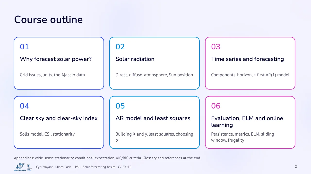
Text of the slide
01
Why forecast solar power?
Grid issues, units, the Ajaccio data
04
Clear sky and clear-sky index
Solis model, CSI, stationarity
Appendices: wide-sense stationarity, conditional expectation, AIC/BIC criteria. Glossary and references at the end.
02 · Solar radiation
Direct, diffuse, atmosphere, Sun position
05
AR model and least squares
Building X and y, least squares, choosing p
03
Time series and forecasting
Components, horizon, a first AR(1) model
06
Evaluation, ELM and online learning
Persistence, metrics, ELM, sliding window, frugality
3 Project objectives
Text of the slide
Context
Solar irradiance is intermittent (clouds).
The power grid must anticipate photovoltaic production.
Need: reliable short-term forecasts (here 1 h).
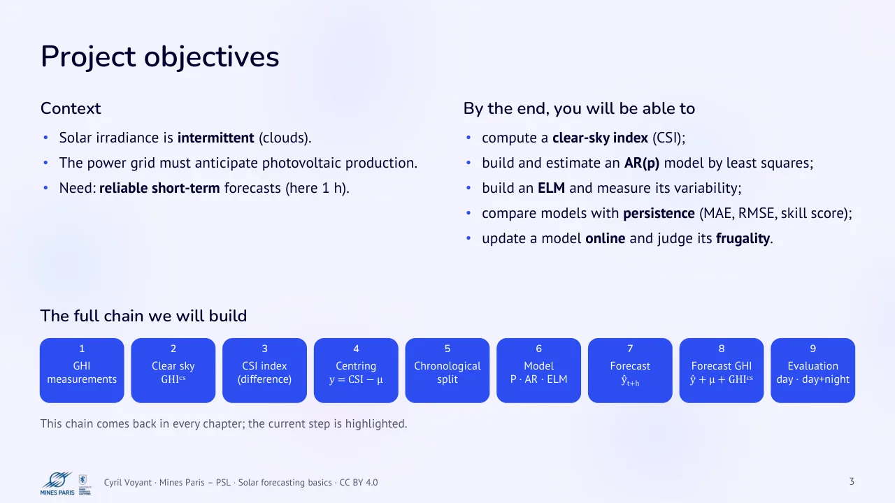
The full chain we will build
1 · 2 · 3 · GHI · measurements · Clear sky · GHIcs · CSI index · (difference)
This chain comes back in every chapter; the current step is highlighted.
By the end, you will be able to
compute a clear-sky index (CSI);
build and estimate an AR(p) model by least squares;
build an ELM and measure its variability;
compare models with persistence (MAE, RMSE, skill score);
update a model online and judge its frugality.
4 · 5 · 6 · 7 · Centring
y = CSI − μ
Chronological · split · Model
P · AR · ELM
Forecast · ŷt+h · 8 · 9 · Forecast GHI
ŷ + μ + GHIcs
Evaluation · day · day+night
4 Notation (used throughout the course)
Text of the slide
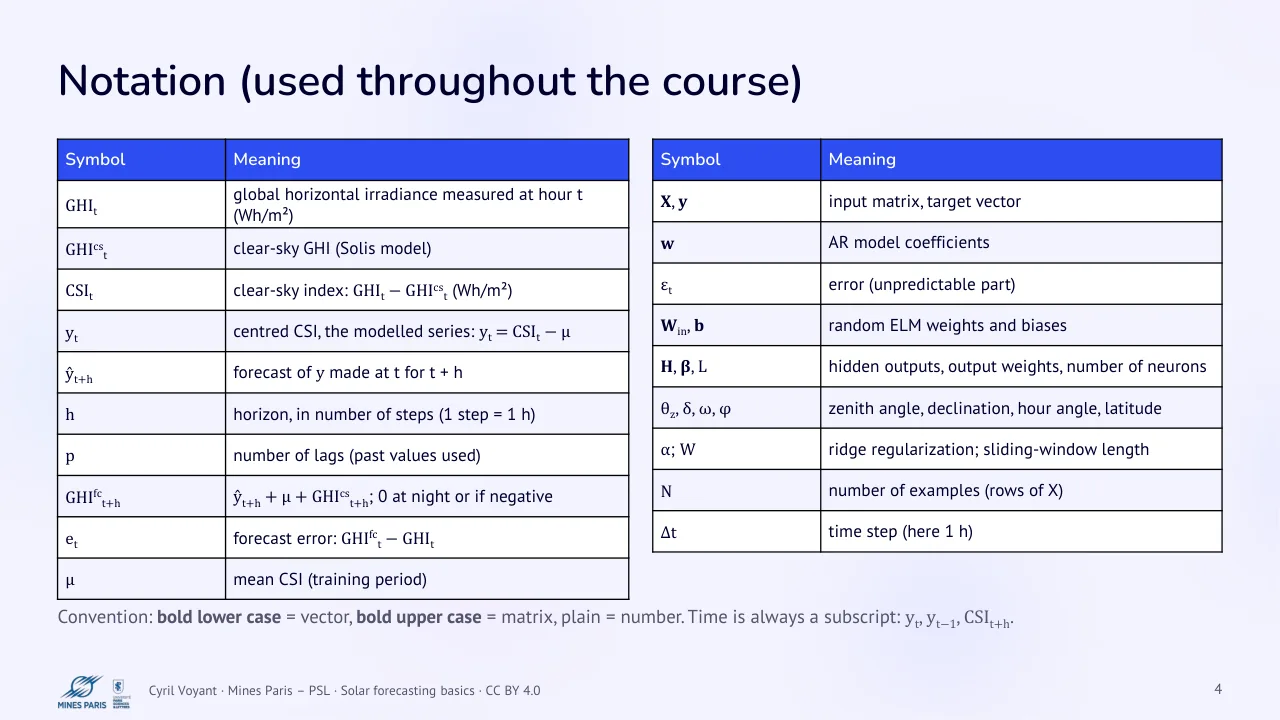
| Symbol | Meaning |
|---|---|
| GHIt | global horizontal irradiance measured at hour t (Wh/m²) |
| GHIcst | clear-sky GHI (Solis model) |
| CSIt | clear-sky index: GHIt − GHIcst (Wh/m²) |
| yt | centred CSI, the modeled series: yt = CSIt − μ |
| ŷt+h | forecast of y made at t for t + h |
| h | horizon, in number of steps (1 step = 1 h) |
| p | number of lags (past values used) |
| GHIfct+h | ŷt+h + μ + GHIcst+h; 0 at night or if negative |
| et | forecast error: GHIfct − GHIt |
| μ | mean CSI (training period) |
Convention: bold lower case = vector, bold upper case = matrix, plain = number. Time is always a subscript: yt, yt−1, CSIt+h.
| Symbol | Meaning |
|---|---|
| X, y | input matrix, target vector |
| w | AR model coefficients |
| εt | error (unpredictable part) |
| Win, b | random ELM weights and biases |
| H, β, L | hidden outputs, output weights, number of neurons |
| θz, δ, ω, φ | zenith angle, declination, hour angle, latitude |
| α; W | ridge regularization; sliding-window length |
| N | number of examples (rows of X) |
| Δt | time step (here 1 h) |
1 · Why forecast solar power?
5 Why forecast? Grid and solar production
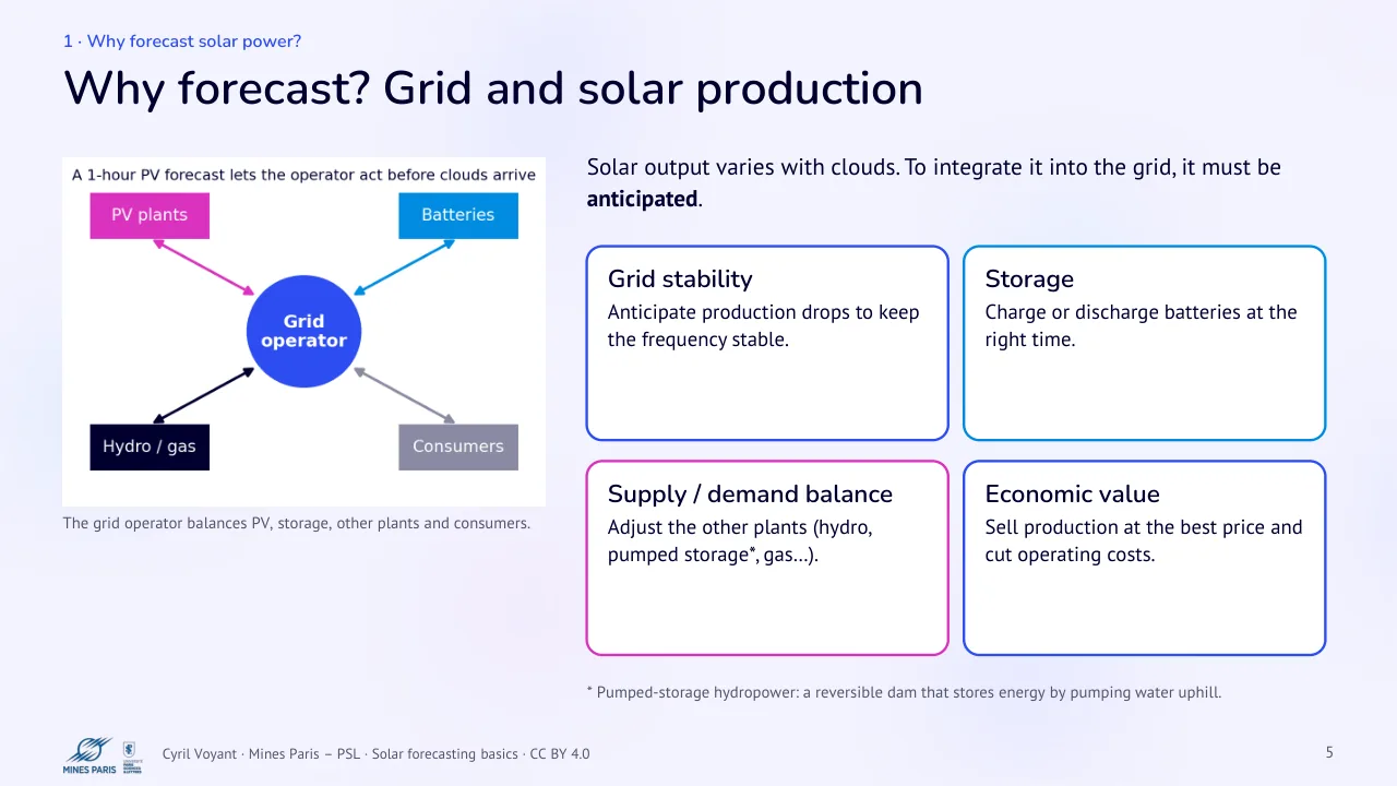
Text of the slide
The grid operator balances PV, storage, other plants and consumers.
Solar output varies with clouds. To integrate it into the grid, it must be anticipated.
Grid stability
Anticipate production drops to keep the frequency stable.
Supply / demand balance
Adjust the other plants (hydro, pumped storage*, gas…).
* Pumped-storage hydropower: a reversible dam that stores energy by pumping water uphill.
Storage
Charge or discharge batteries at the right time.
Economic value
Sell production at the best price and cut operating costs.
6 Irradiance, irradiation and photovoltaic output
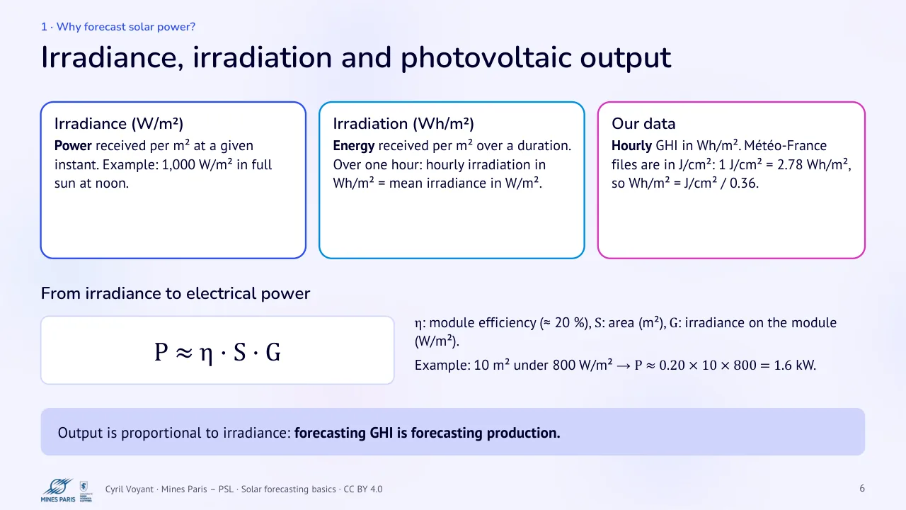
Text of the slide
Irradiance (W/m²)
Power received per m² at a given instant. Example: 1,000 W/m² in full sun at noon.
From irradiance to electrical power
P ≈ η · S · G
Output is proportional to irradiance: forecasting GHI is forecasting production.
Irradiation (Wh/m²)
Energy received per m² over a duration. Over one hour: hourly irradiation in Wh/m² = mean irradiance in W/m².
η: module efficiency (≈ 20 %), S: area (m²), G: irradiance on the module (W/m²).
Example: 10 m² under 800 W/m² → P ≈ 0.20 × 10 × 800 = 1.6 kW.
Our data
Hourly GHI in Wh/m². Météo-France files are in J/cm²: 1 J/cm² = 2.78 Wh/m², so Wh/m² = J/cm² / 0.36.
7 The dataset: Ajaccio, 1998–2007
Text of the slide
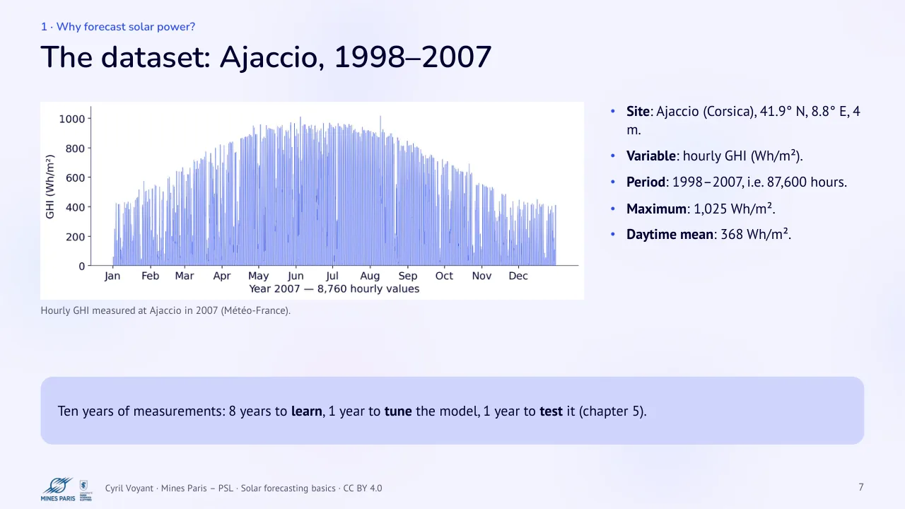
Hourly GHI measured at Ajaccio in 2007 (Météo-France).
Ten years of measurements: 8 years to learn, 1 year to tune the model, 1 year to test it (chapter 5).
Site: Ajaccio (Corsica), 41.9° N, 8.8° E, 4 m.
Variable: hourly GHI (Wh/m²).
Period: 1998–2007, i.e. 87,600 hours.
Maximum: 1,025 Wh/m².
Daytime mean: 368 Wh/m².
2 · Solar radiation
8 Components of global radiation
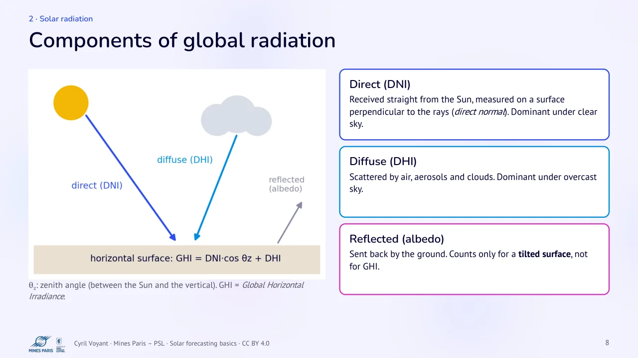
Text of the slide
θz: zenith angle (between the Sun and the vertical). GHI = Global Horizontal Irradiance.
Direct (DNI)
Received straight from the Sun, measured on a surface perpendicular to the rays (direct normal). Dominant under clear sky.
Diffuse (DHI)
Scattered by air, aerosols and clouds. Dominant under overcast sky.
Reflected (albedo)
Sent back by the ground. Counts only for a tilted surface, not for GHI.
9 Crossing the atmosphere
Text of the slide
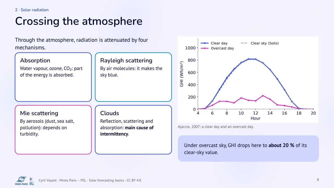
Through the atmosphere, radiation is attenuated by four mechanisms.
Absorption · Rayleigh scattering
Water vapour, ozone, CO₂: part of the energy is absorbed.
By air molecules: it makes the sky blue.
Mie scattering · Clouds
By aerosols (dust, sea salt, pollution): depends on turbidity.
Reflection, scattering and absorption: main cause of intermittency.
Ajaccio, 2007: a clear day and an overcast day.
Under overcast sky, GHI drops here to about 20 % of its clear-sky value.
10 The position of the Sun
Text of the slide
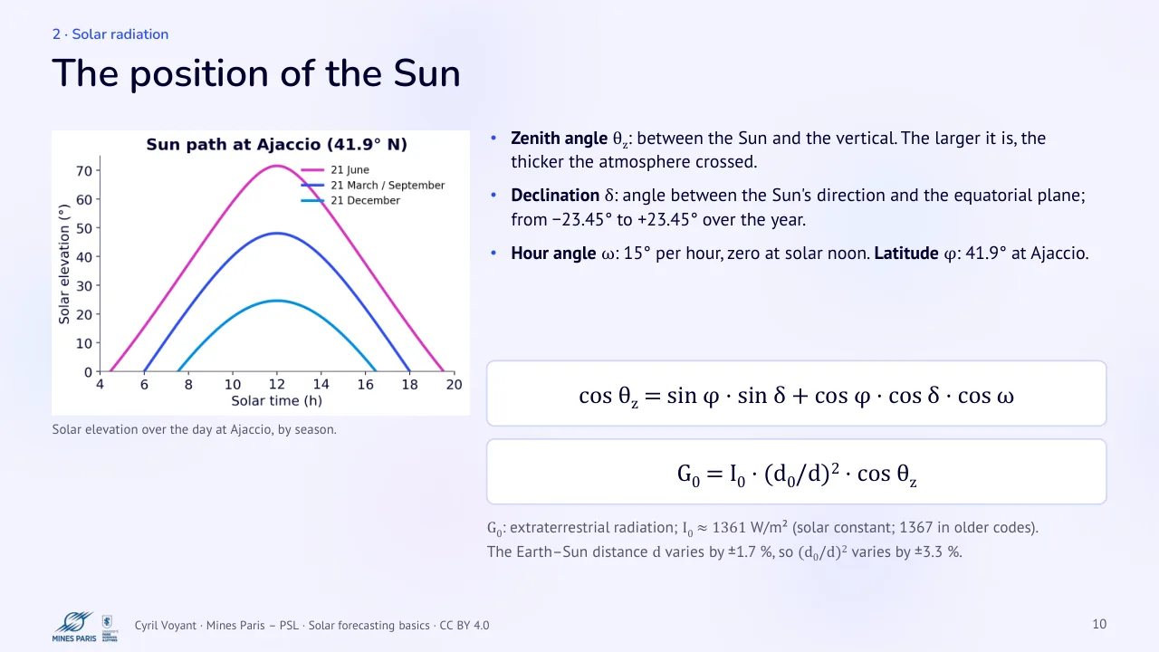
Solar elevation over the day at Ajaccio, by season.
Zenith angle θz: between the Sun and the vertical. The larger it is, the thicker the atmosphere crossed.
Declination δ: angle between the Sun's direction and the equatorial plane; from −23.45° to +23.45° over the year.
Hour angle ω: 15° per hour, zero at solar noon. Latitude φ: 41.9° at Ajaccio.
cos θz = sin φ · sin δ + cos φ · cos δ · cos ω
G0 = I0 · (d0/d)2 · cos θz
G0: extraterrestrial radiation; I0 ≈ 1361 W/m² (solar constant; 1367 in older codes).
The Earth–Sun distance d varies by ±1.7 %, so (d0/d)2 varies by ±3.3 %.
11 The double seasonality of GHI
Text of the slide
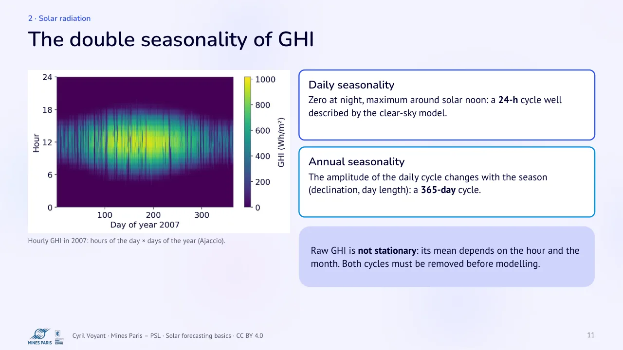
Hourly GHI in 2007: hours of the day × days of the year (Ajaccio).
Daily seasonality
Zero at night, maximum around solar noon: a 24-h cycle well described by the clear-sky model.
Annual seasonality
The amplitude of the daily cycle changes with the season (declination, day length): a 365-day cycle.
Raw GHI is not stationary: its mean depends on the hour and the month. Both cycles must be removed before modeling.
3 · Time series and forecasting
12 What is a time series?
Text of the slide
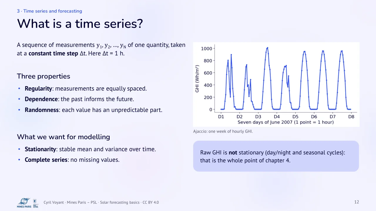
A sequence of measurements y1, y2, …, yN of one quantity, taken at a constant time step Δt. Here Δt = 1 h.
Three properties
Regularity: measurements are equally spaced.
Dependence: the past informs the future.
Randomness: each value has an unpredictable part.
What we want for modeling
Stationarity: stable mean and variance over time.
Complete series: no missing values.
Ajaccio: one week of hourly GHI.
Raw GHI is not stationary (day/night and seasonal cycles): that is the whole point of chapter 4.
13 Components of a time series
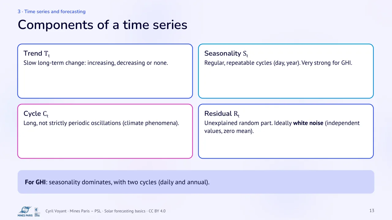
Text of the slide
Trend Tt
Slow long-term change: increasing, decreasing or none.
Cycle Ct
Long, not strictly periodic oscillations (climate phenomena).
For GHI: seasonality dominates, with two cycles (daily and annual).
Seasonality St
Regular, repeatable cycles (day, year). Very strong for GHI.
Residual Rt
Unexplained random part. Ideally white noise (independent values, zero mean).
14 Decomposing a time series
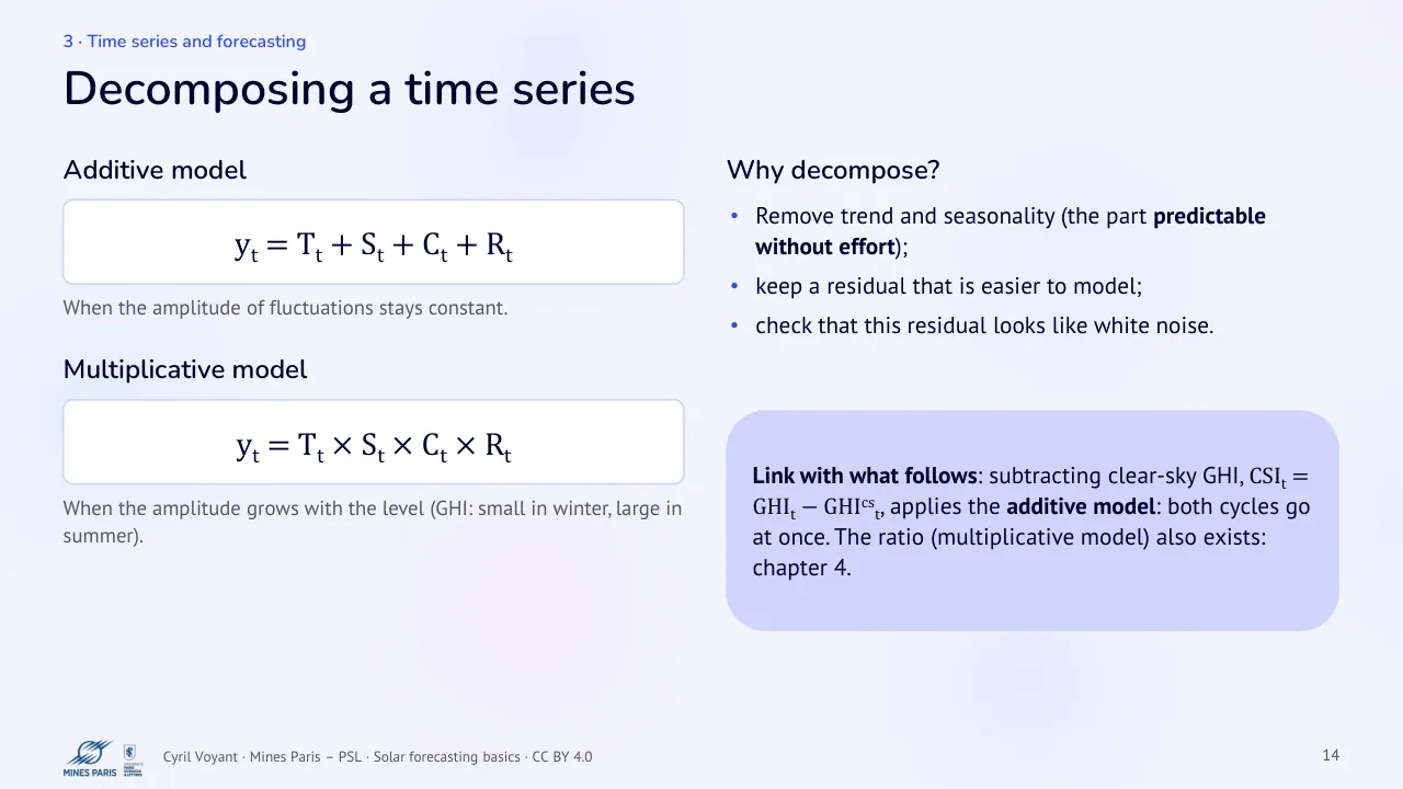
Text of the slide
Additive model
yt = Tt + St + Ct + Rt
When the amplitude of fluctuations stays constant.
Multiplicative model
yt = Tt × St × Ct × Rt
When the amplitude grows with the level (GHI: small in winter, large in summer).
Why decompose?
Remove trend and seasonality (the part predictable without effort);
keep a residual that is easier to model;
check that this residual looks like white noise.
Link with what follows: subtracting clear-sky GHI, CSIt = GHIt − GHIcst, applies the additive model: both cycles go at once. The ratio (multiplicative model) also exists: chapter 4.
15 Horizon, time step and types of forecast
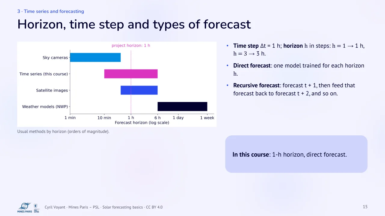
Text of the slide
Usual methods by horizon (orders of magnitude).
Time step Δt = 1 h; horizon h in steps: h = 1 → 1 h, h = 3 → 3 h.
Direct forecast: one model trained for each horizon h.
Recursive forecast: forecast t + 1, then feed that forecast back to forecast t + 2, and so on.
In this course: 1-h horizon, direct forecast.
16 Forecasting: a predictable part and an error
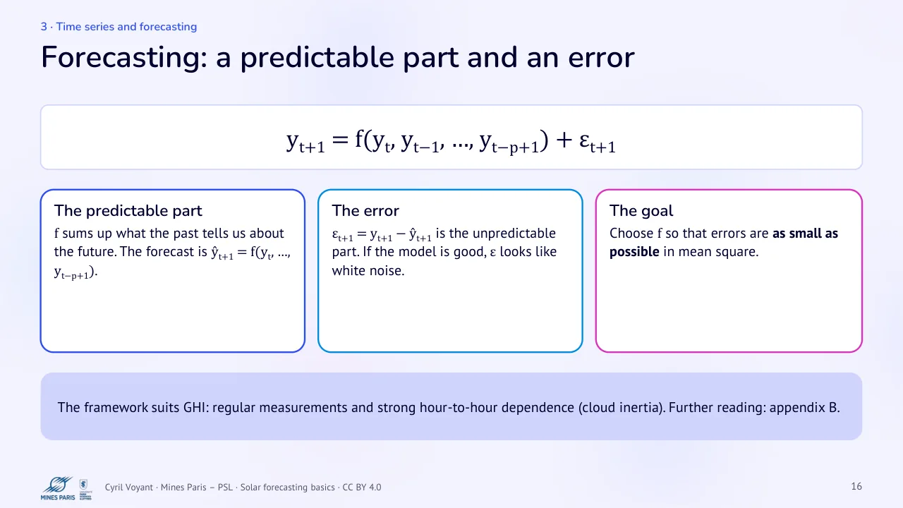
Text of the slide
yt+1 = f(yt, yt−1, …, yt−p+1) + εt+1
The predictable part
f sums up what the past tells us about the future. The forecast is ŷt+1 = f(yt, …, yt−p+1).
The framework suits GHI: regular measurements and strong hour-to-hour dependence (cloud inertia). Further reading: appendix B.
The error
εt+1 = yt+1 − ŷt+1 is the unpredictable part. If the model is good, ε looks like white noise.
The goal
Choose f so that errors are as small as possible in mean square.
17 A first example: the AR(1) model, with numbers
Text of the slide
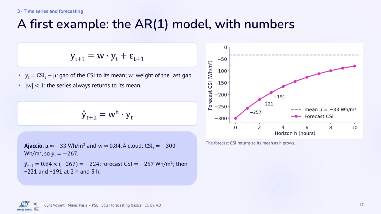
yt+1 = w · yt + εt+1
yt = CSIt − μ: gap of the CSI to its mean; w: weight of the last gap.
|w| < 1: the series always returns to its mean.
ŷt+h = wh · yt
Ajaccio: μ ≈ −33 Wh/m² and w ≈ 0.84. A cloud: CSIt = −300 Wh/m², so yt = −267.
ŷt+1 = 0.84 × (−267) = −224: forecast CSI = −257 Wh/m²; then −221 and −191 at 2 h and 3 h.
The forecast CSI returns to its mean as h grows.
4 · Clear sky and clear-sky index
18 The clear-sky model
Text of the slide
What is it?
The GHI one would measure without clouds, given the Sun's position and a clear atmosphere.
Inputs
site position (latitude, longitude, altitude);
Sun position (θz);
water vapour and aerosols (AOD: aerosol optical depth).
Role: GHIcst is the reference used to remove the day/night and seasonal cycles.
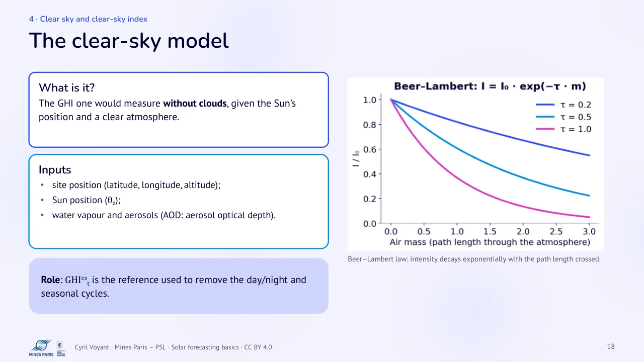
Beer–Lambert law: intensity decays exponentially with the path length crossed.
19 The Solis model
Text of the slide
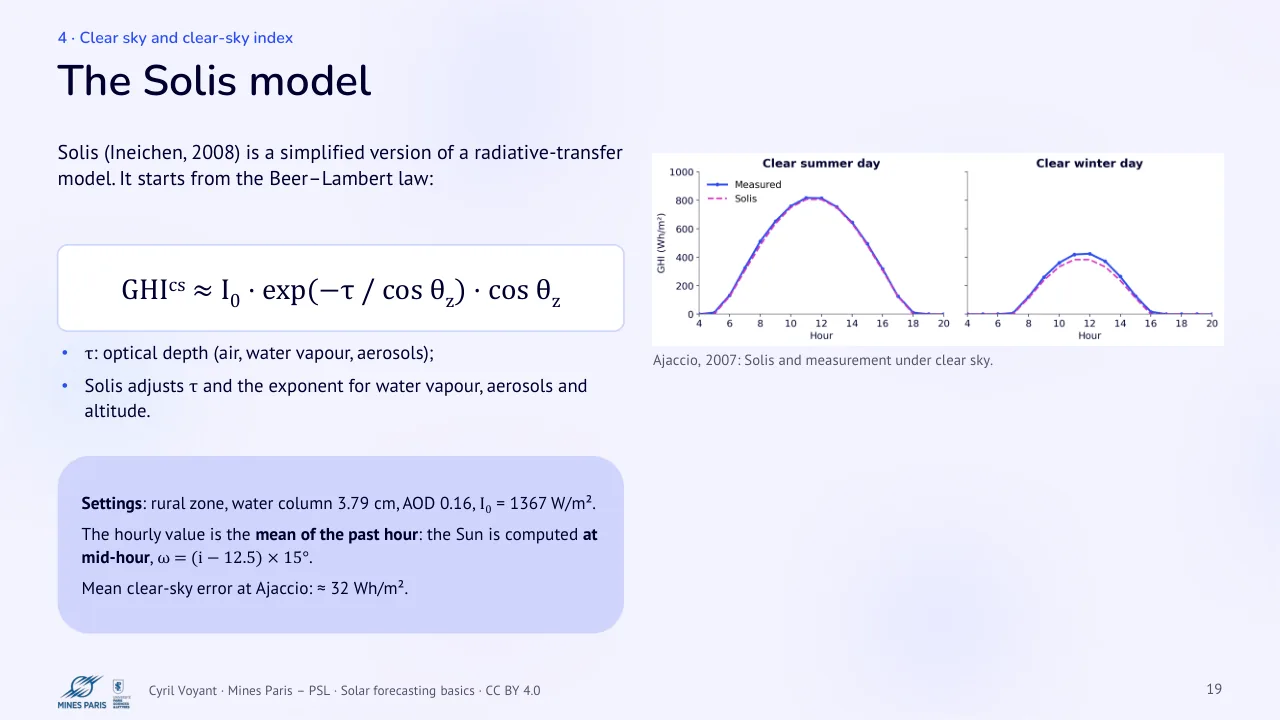
Solis (Ineichen, 2008) is a simplified version of a radiative-transfer model. It starts from the Beer–Lambert law:
GHIcs ≈ I0 · exp(−τ / cos θz) · cos θz
τ: optical depth (air, water vapour, aerosols);
Solis adjusts τ and the exponent for water vapour, aerosols and altitude.
Settings: rural zone, water column 3.79 cm, AOD 0.16, I0 = 1367 W/m².
The hourly value is the mean of the past hour: the Sun is computed at mid-hour, ω = (i − 12.5) × 15°.
Mean clear-sky error at Ajaccio: ≈ 32 Wh/m².
Ajaccio, 2007: Solis and measurement under clear sky.
20 Stationarizing: the clear-sky index (CSI)
Text of the slide
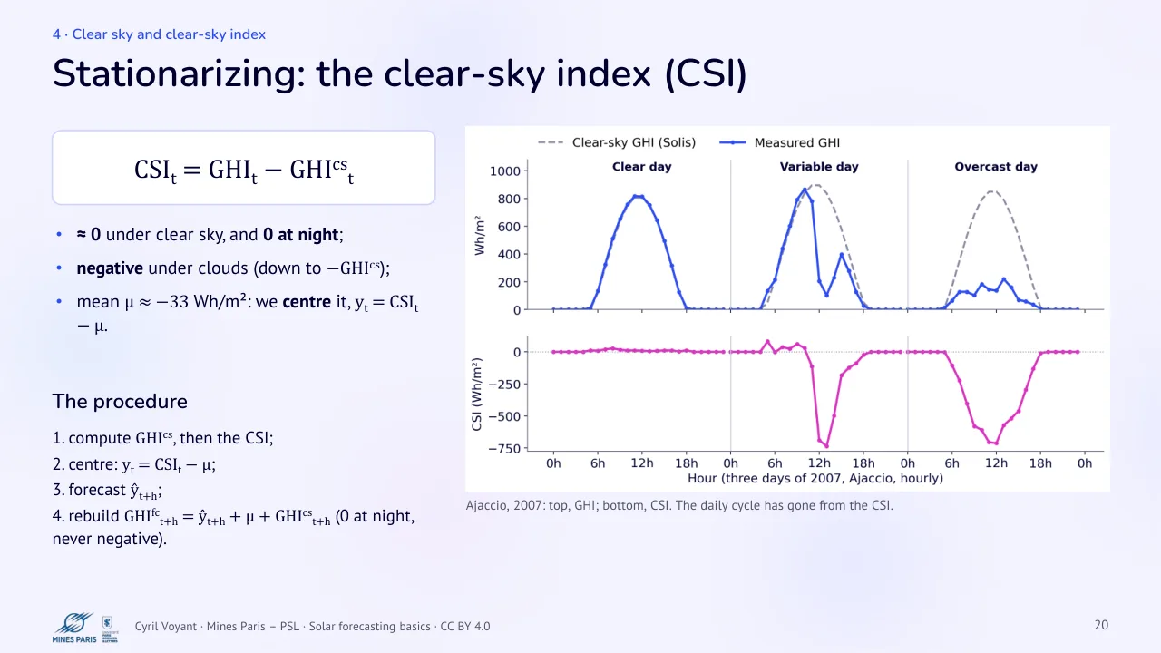
CSIt = GHIt − GHIcst
≈ 0 under clear sky, and 0 at night;
negative under clouds (down to −GHIcs);
mean μ ≈ −33 Wh/m²: we center it, yt = CSIt − μ.
The procedure
- compute GHIcs, then the CSI;
- center: yt = CSIt − μ;
- forecast ŷt+h;
- rebuild GHIfct+h = ŷt+h + μ + GHIcst+h (0 at night, never negative).
Ajaccio, 2007: top, GHI; bottom, CSI. The daily cycle has gone from the CSI.
21 Two ways to stationarize
Text of the slide
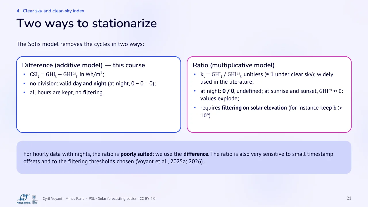
The Solis model removes the cycles in two ways:
Difference (additive model), this course
CSIt = GHIt − GHIcst, in Wh/m²;
no division: valid day and night (at night, 0 − 0 = 0);
all hours are kept, no filtering.
For hourly data with nights, the ratio is poorly suited: we use the difference. The ratio is also very sensitive to small timestamp offsets and to the filtering thresholds chosen (Voyant et al., 2025a; 2026).
Ratio (multiplicative model)
kt = GHIt / GHIcst, unitless (≈ 1 under clear sky); widely used in the literature;
at night: 0 / 0, undefined; at sunrise and sunset, GHIcs ≈ 0: values explode;
requires filtering on solar elevation (for instance keep h > 10°).
22 Is the CSI stationary?
Text of the slide
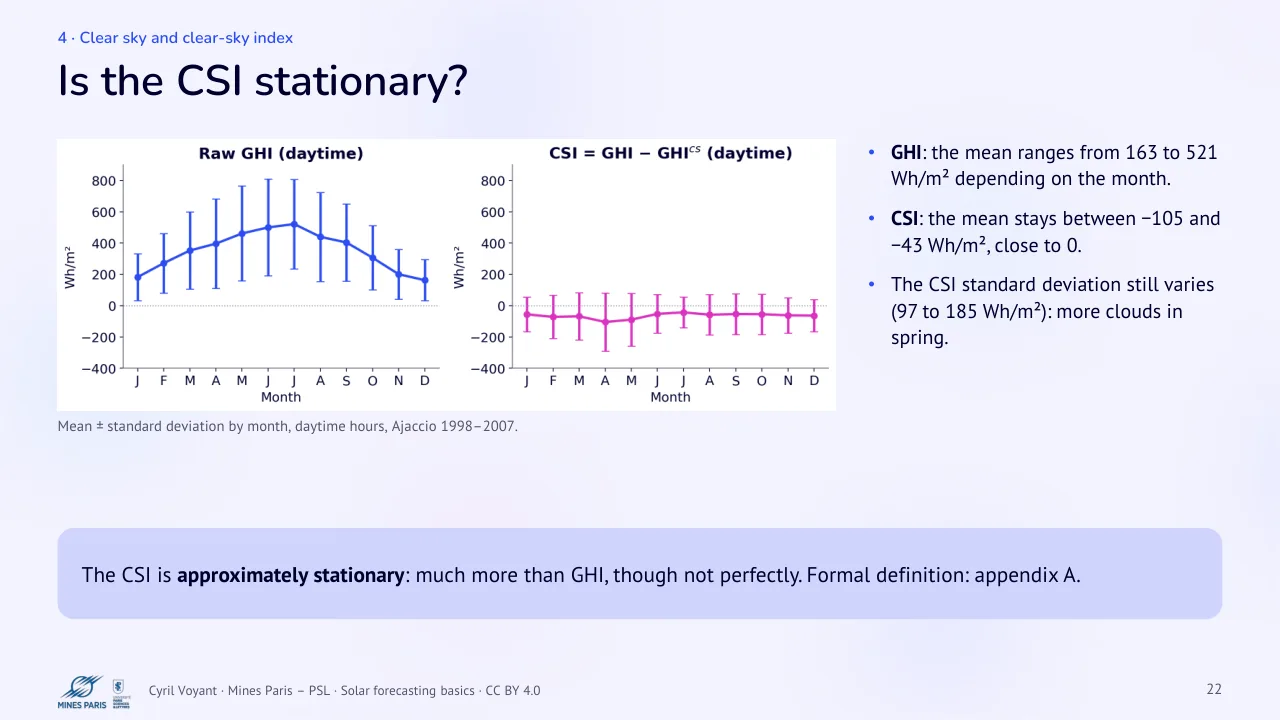
Mean ± standard deviation by month, daytime hours, Ajaccio 1998–2007.
The CSI is approximately stationary: much more than GHI, though not perfectly. Formal definition: appendix A.
GHI: the mean ranges from 163 to 521 Wh/m² depending on the month.
CSI: the mean stays between −105 and −43 Wh/m², close to 0.
The CSI standard deviation still varies (97 to 185 Wh/m²): more clouds in spring.
23 Site variability: the sCV
Text of the slide
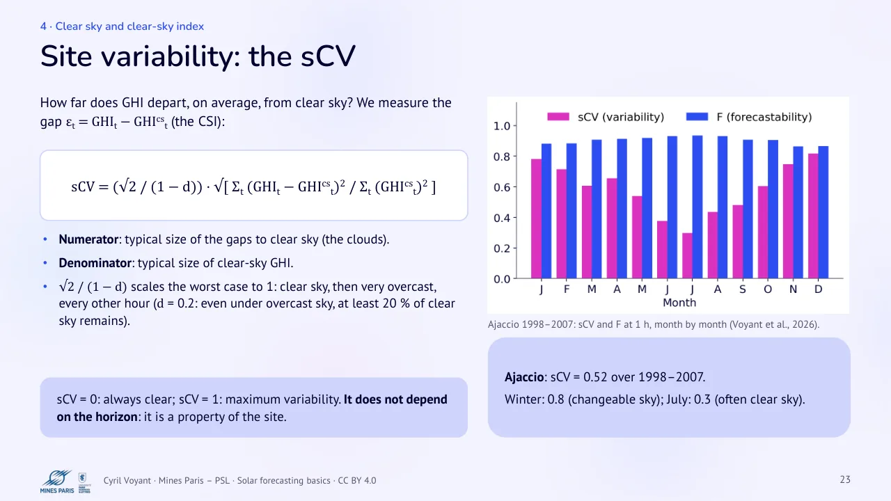
How far does GHI depart, on average, from clear sky? We measure the gap εt = GHIt − GHIcst (the CSI):
sCV = (√2 / (1 − d)) · √[ Σt (GHIt − GHIcst)2 / Σt (GHIcst)2 ]
Numerator: typical size of the gaps to clear sky (the clouds).
Denominator: typical size of clear-sky GHI.
√2 / (1 − d) scales the worst case to 1: clear sky, then very overcast, every other hour (d = 0.2: even under overcast sky, at least 20 % of clear sky remains).
sCV = 0: always clear; sCV = 1: maximum variability. It does not depend on the horizon: it is a property of the site.
Ajaccio 1998–2007: sCV and F at 1 h, month by month (Voyant et al., 2026).
Ajaccio: sCV = 0.52 over 1998–2007.
Winter: 0.8 (changeable sky); July: 0.3 (often clear sky).
24 Forecastability: F depends on the horizon
Text of the slide
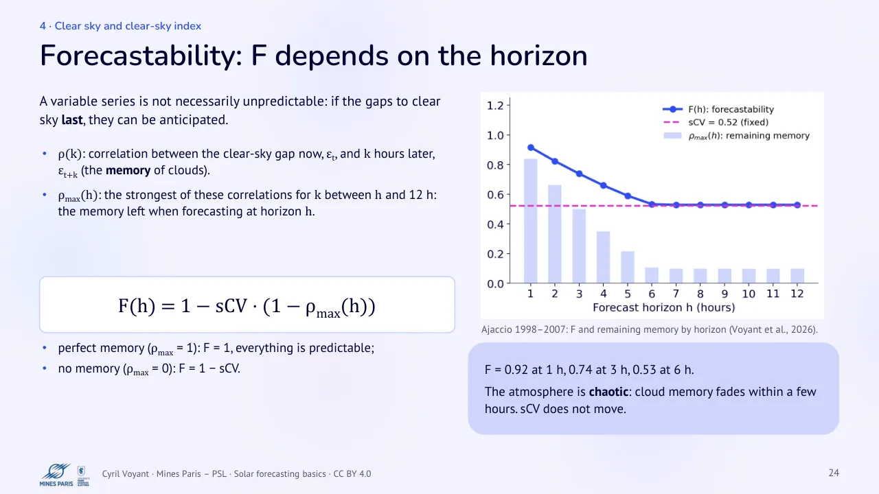
A variable series is not necessarily unpredictable: if the gaps to clear sky last, they can be anticipated.
ρ(k): correlation between the clear-sky gap now, εt, and k hours later, εt+k (the memory of clouds).
ρmax(h): the strongest of these correlations for k between h and 12 h: the memory left when forecasting at horizon h.
F(h) = 1 − sCV · (1 − ρmax(h))
perfect memory (ρmax = 1): F = 1, everything is predictable;
no memory (ρmax = 0): F = 1 − sCV.
Ajaccio 1998–2007: F and remaining memory by horizon (Voyant et al., 2026).
F = 0.92 at 1 h, 0.74 at 3 h, 0.53 at 6 h.
The atmosphere is chaotic: cloud memory fades within a few hours. sCV does not move.
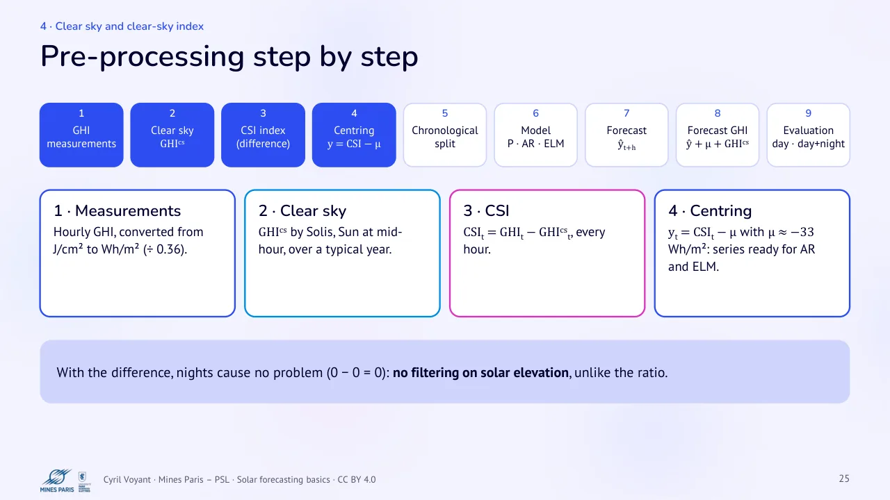
25 Pre-processing step by step
Text of the slide
1 · 2 · 3 · GHI · measurements · Clear sky · GHIcs · CSI index · (difference) · 1 · Measurements
2 · Clear sky
Hourly GHI, converted from J/cm² to Wh/m² (÷ 0.36).
GHIcs by Solis, Sun at mid-hour, over a typical year.
With the difference, nights cause no problem (0 − 0 = 0): no filtering on solar elevation, unlike the ratio.
4 · 5 · 6 · 7 · Centring
y = CSI − μ
Chronological · split · Model
P · AR · ELM
Forecast · ŷt+h · 3 · CSI
CSIt = GHIt − GHIcst, every hour.
8 · 9 · Forecast GHI
ŷ + μ + GHIcs
Evaluation · day · day+night · 4 · Centring
yt = CSIt − μ with μ ≈ −33 Wh/m²: series ready for AR and ELM.
5 · AR model and least squares
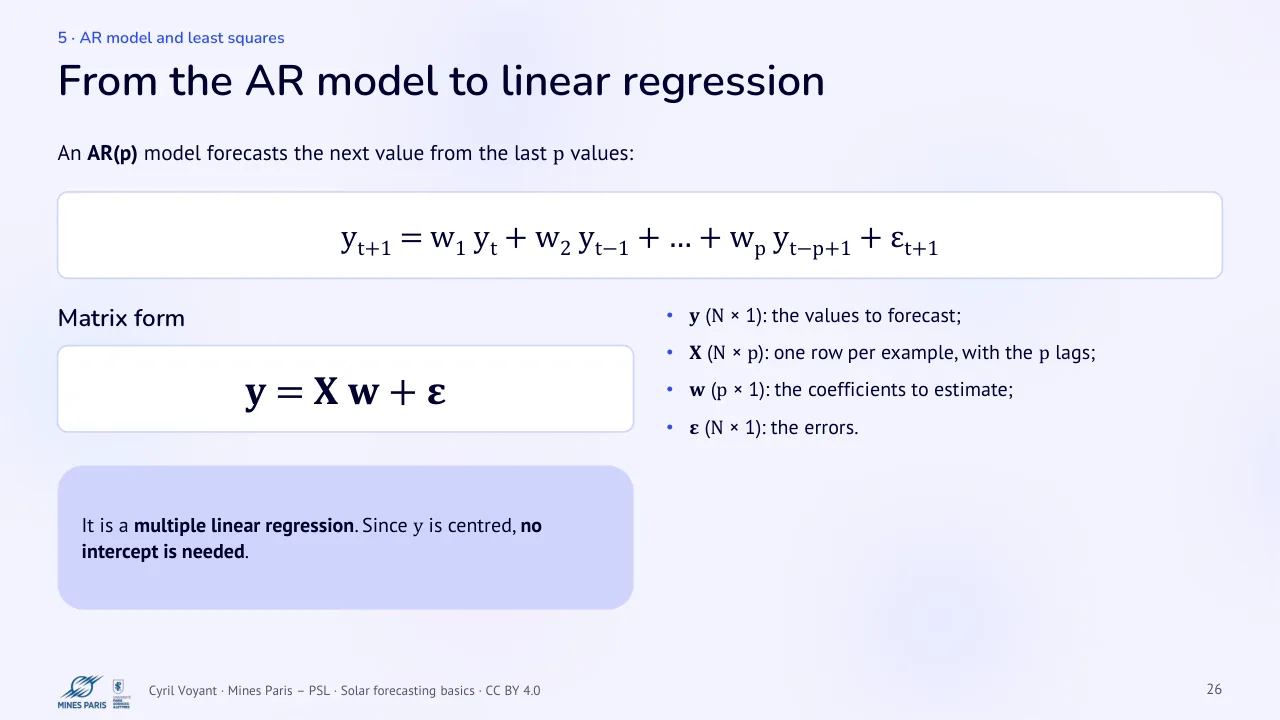
26 From the AR model to linear regression
Text of the slide
An AR(p) model forecasts the next value from the last p values:
yt+1 = w1 yt + w2 yt−1 + … + wp yt−p+1 + εt+1
Matrix form
y = X w + ε
It is a multiple linear regression. Since y is centred, no intercept is needed.
y (N × 1): the values to forecast;
X (N × p): one row per example, with the p lags;
w (p × 1): the coefficients to estimate;
ε (N × 1): the errors.
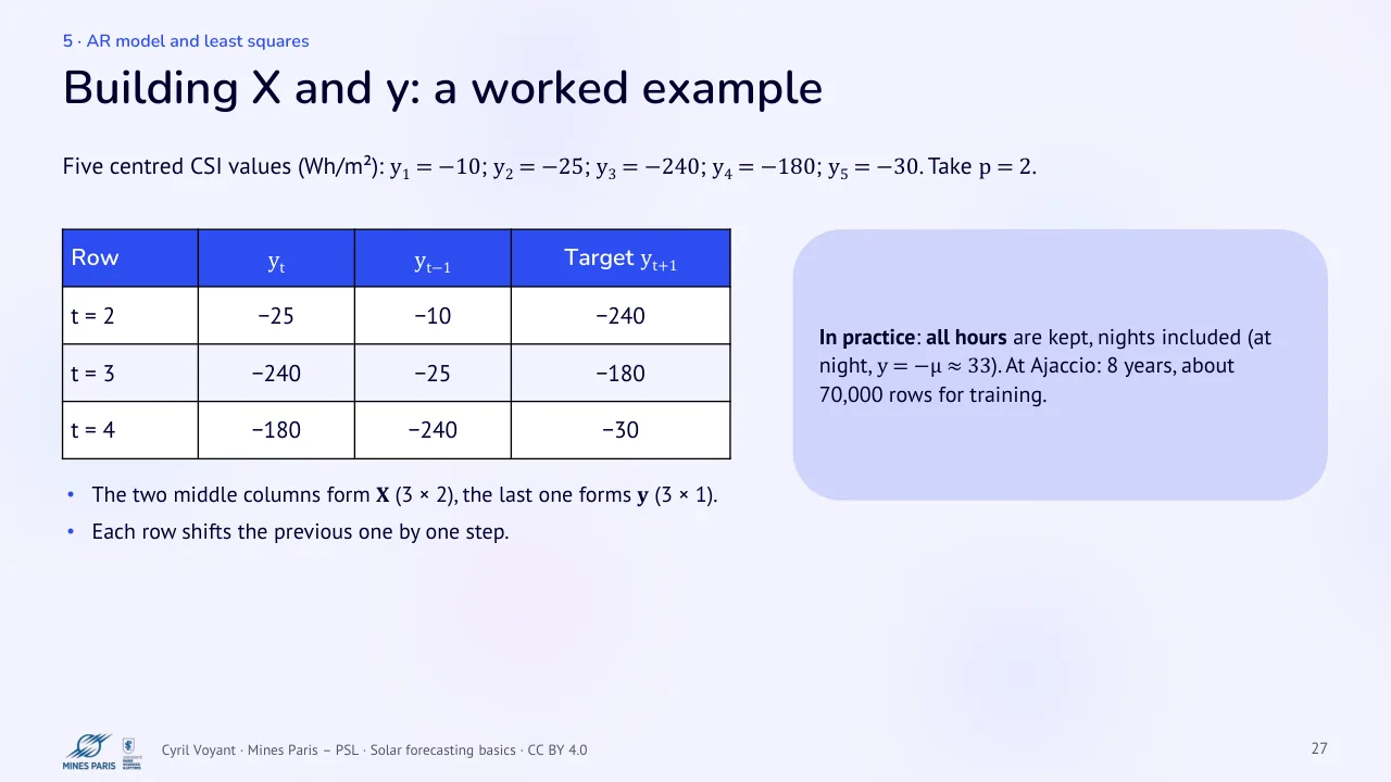
27 Building X and y: a worked example
Text of the slide
Five centred CSI values (Wh/m²): y1 = −10; y2 = −25; y3 = −240; y4 = −180; y5 = −30. Take p = 2.
| Row | yt | yt−1 | Target yt+1 |
|---|---|---|---|
| t = 2 | −25 | −10 | −240 |
| t = 3 | −240 | −25 | −180 |
| t = 4 | −180 | −240 | −30 |
The two middle columns form X (3 × 2), the last one forms y (3 × 1).
Each row shifts the previous one by one step.
In practice: all hours are kept, nights included (at night, y = −μ ≈ 33). At Ajaccio: 8 years, about 70,000 rows for training.
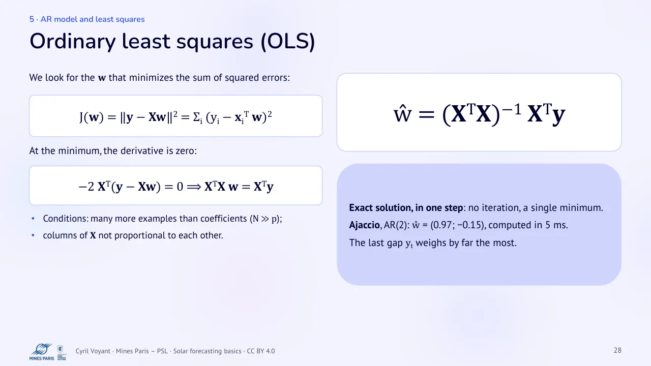
28 Ordinary least squares (OLS)
Text of the slide
We look for the w that minimizes the sum of squared errors:
J(w) = ‖y − Xw‖2 = Σi (yi − xiT w)2
At the minimum, the derivative is zero:
−2 XT(y − Xw) = 0 ⟹ XTX w = XTy
Conditions: many more examples than coefficients (N ≫ p);
columns of X not proportional to each other.
ŵ = (XTX)−1 XTy
Exact solution, in one step: no iteration, a single minimum.
Ajaccio, AR(2): ŵ = (0.97; −0.15), computed in 5 ms.
The last gap yt weighs by far the most.
29 Geometric interpretation
Text of the slide
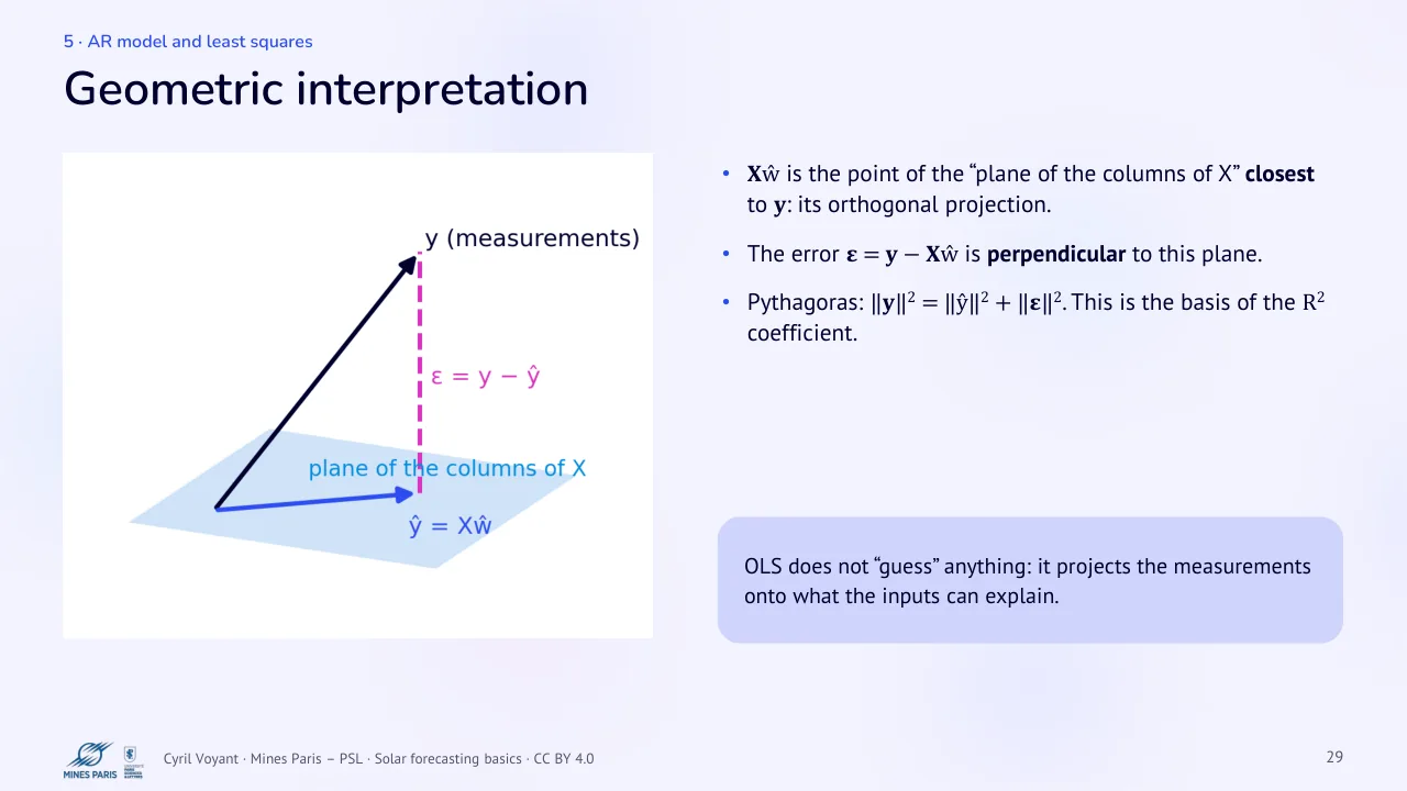
Xŵ is the point of the “plane of the columns of X” closest to y: its orthogonal projection.
The error ε = y − Xŵ is perpendicular to this plane.
Pythagoras: ‖y‖2 = ‖ŷ‖2 + ‖ε‖2. This is the basis of the R2 coefficient.
OLS does not “guess” anything: it projects the measurements onto what the inputs can explain.
30 Training, validation, test
Text of the slide
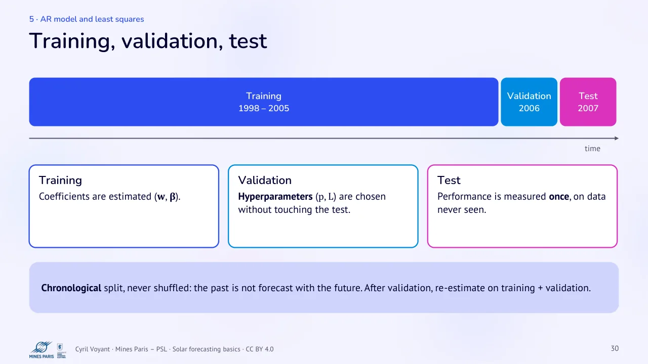
Training · 1998 – 2005 · Training
Coefficients are estimated (w, β).
Chronological split, never shuffled: the past is not forecast with the future. After validation, re-estimate on training + validation.
Validation
Hyperparameters (p, L) are chosen without touching the test.
Validation · 2006 · Test · 2007 · time · Test
Performance is measured once, on data never seen.
31 Choosing p (1/3): autocorrelation (ACF)
Text of the slide
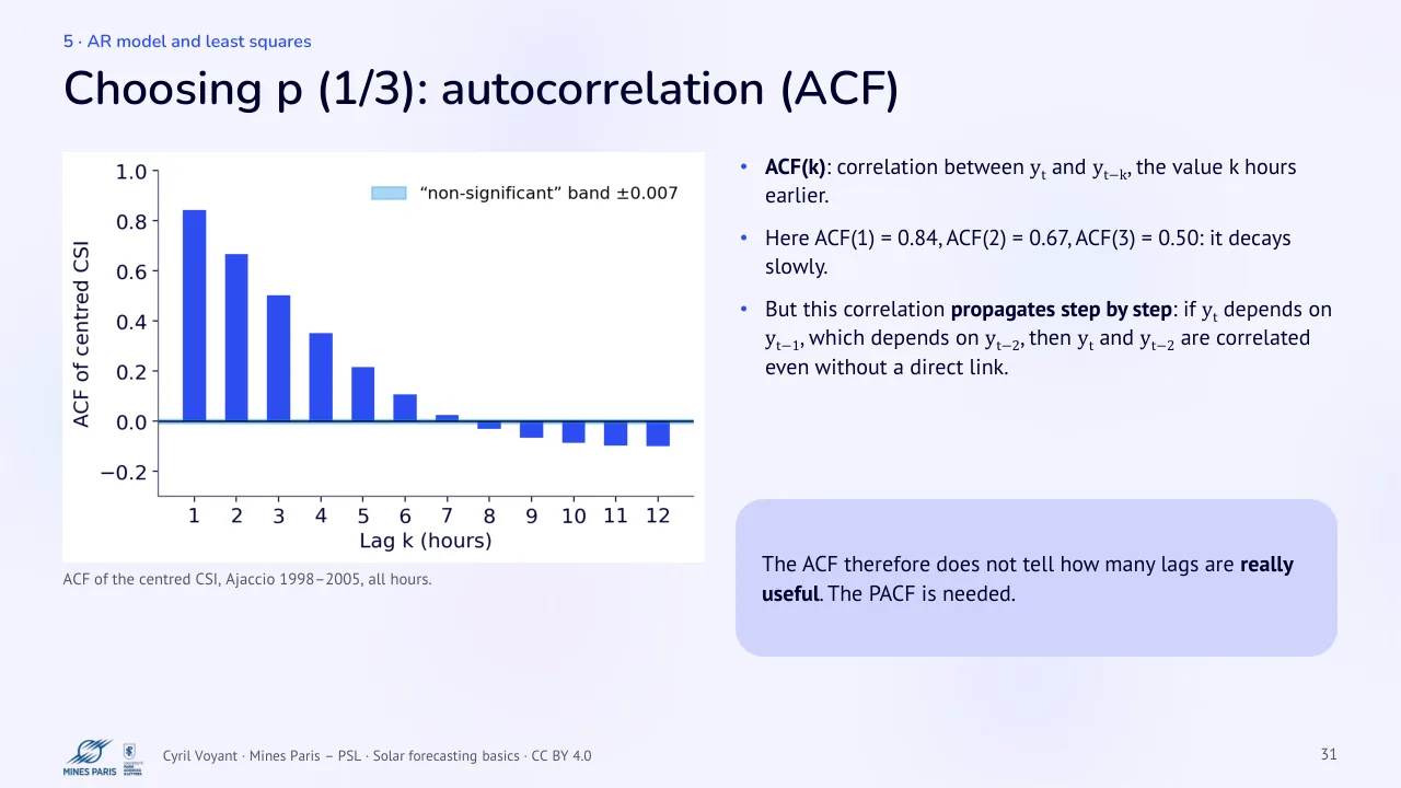
ACF of the centred CSI, Ajaccio 1998–2005, all hours.
ACF(k): correlation between yt and yt−k, the value k hours earlier.
Here ACF(1) = 0.84, ACF(2) = 0.67, ACF(3) = 0.50: it decays slowly.
But this correlation propagates step by step: if yt depends on yt−1, which depends on yt−2, then yt and yt−2 are correlated even without a direct link.
The ACF therefore does not tell how many lags are really useful. The PACF is needed.
32 Choosing p (2/3): partial autocorrelation (PACF)
Text of the slide
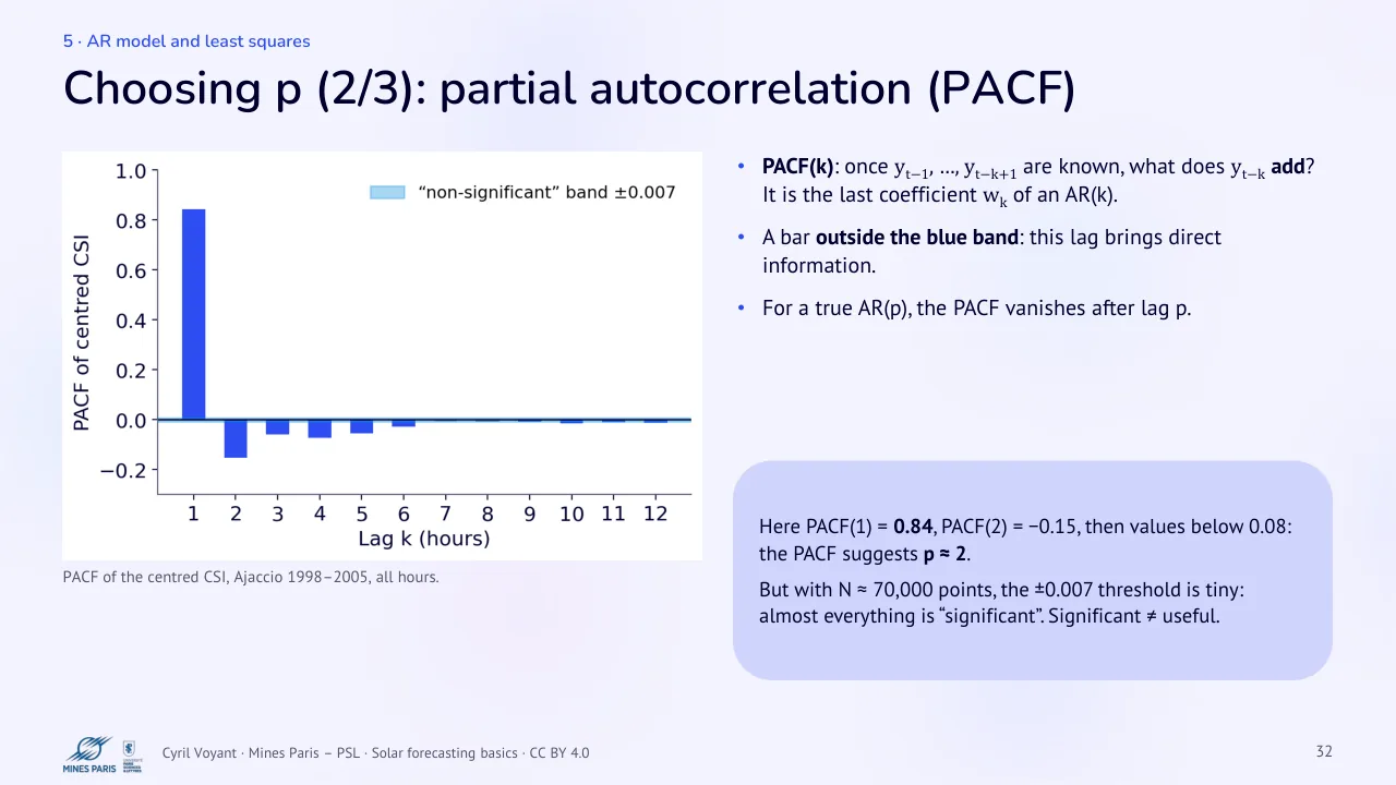
PACF of the centred CSI, Ajaccio 1998–2005, all hours.
PACF(k): once yt−1, …, yt−k+1 are known, what does yt−k add? It is the last coefficient wk of an AR(k).
A bar outside the blue band: this lag brings direct information.
For a true AR(p), the PACF vanishes after lag p.
Here PACF(1) = 0.84, PACF(2) = −0.15, then values below 0.08: the PACF suggests p ≈ 2.
But with N ≈ 70,000 points, the ±0.007 threshold is tiny: almost everything is “significant”. Significant ≠ useful.
33 Choosing p (3/3): filter or wrapper approach
Text of the slide
Filter
look at the data alone, before any model: PACF, AIC / BIC criteria (appendix C);
fast, but indirect.
Wrapper
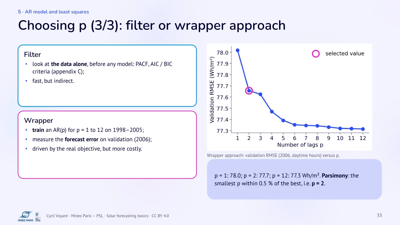
train an AR(p) for p = 1 to 12 on 1998–2005;
measure the forecast error on validation (2006);
driven by the real objective, but more costly.
Wrapper approach: validation RMSE (2006, daytime hours) versus p.
p = 1: 78.0; p = 2: 77.7; p = 12: 77.3 Wh/m². Parsimony: the smallest p within 0.5 % of the best, i.e. p = 2.
34 Summary: forecasting GHI with an AR(p)
Text of the slide
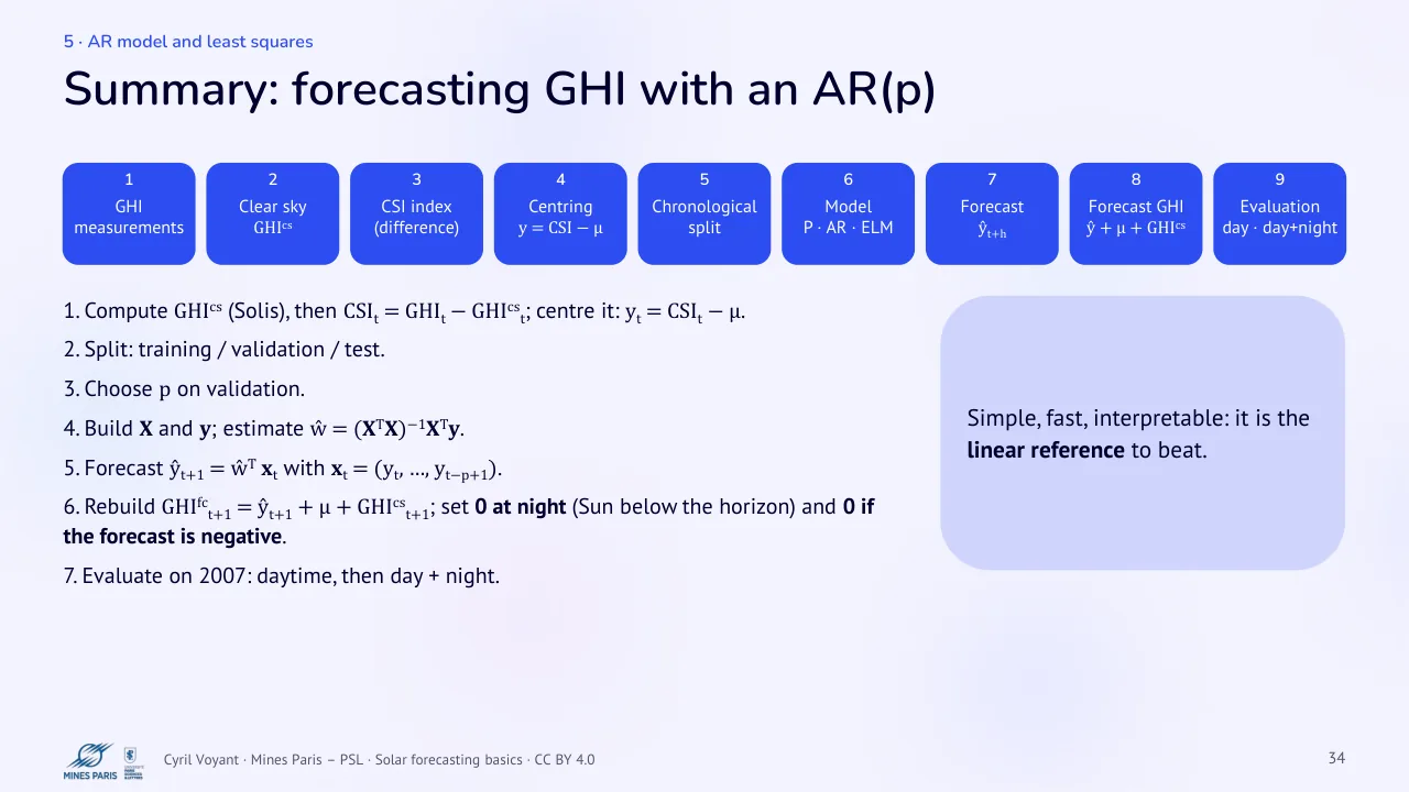
1 · 2 · 3 · GHI · measurements · Clear sky · GHIcs · CSI index · (difference)
- Compute GHIcs (Solis), then CSIt = GHIt − GHIcst; center it: yt = CSIt − μ.
- Split: training / validation / test.
- Choose p on validation.
- Build X and y; estimate ŵ = (XTX)−1XTy.
- Forecast ŷt+1 = ŵT xt with xt = (yt, …, yt−p+1).
- Rebuild GHIfct+1 = ŷt+1 + μ + GHIcst+1; set 0 at night (Sun below the horizon) and 0 if the forecast is negative.
- Evaluate on 2007: daytime, then day + night.
4 · 5 · 6 · 7 · Centring
y = CSI − μ
Chronological · split · Model
P · AR · ELM
Forecast · ŷt+h · 8 · 9 · Forecast GHI
ŷ + μ + GHIcs
Evaluation · day · day+night
Simple, fast, interpretable: it is the linear reference to beat.
6 · Evaluation, ELM and online learning
35 Reference models
Text of the slide
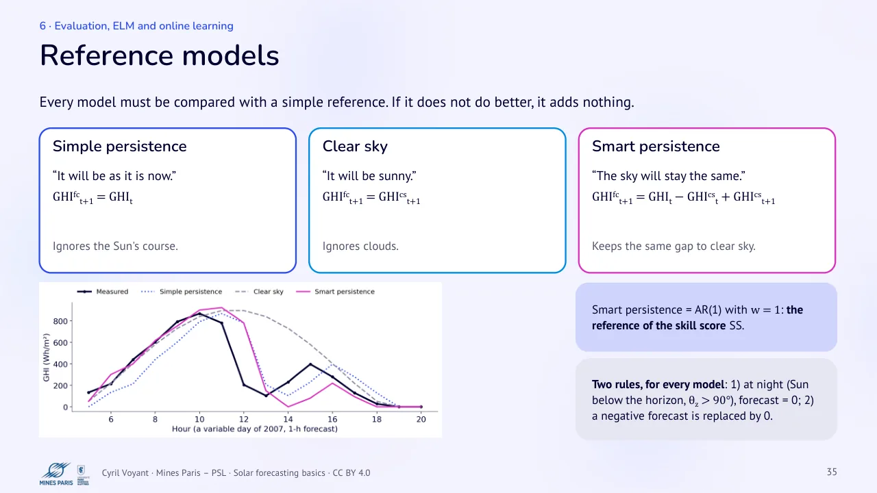
Every model must be compared with a simple reference. If it does not do better, it adds nothing.
Simple persistence
“It will be as it is now.”
GHIfct+1 = GHIt
Ignores the Sun's course.
Clear sky
“It will be sunny.”
GHIfct+1 = GHIcst+1
Ignores clouds.
Smart persistence
“The sky will stay the same.”
GHIfct+1 = GHIt − GHIcst + GHIcst+1
Keeps the same gap to clear sky.
Smart persistence = AR(1) with w = 1: the reference of the skill score SS.
Two rules, for every model: 1) at night (Sun below the horizon, θz > 90°), forecast = 0; 2) a negative forecast is replaced by 0.
36 Measuring the error
Text of the slide
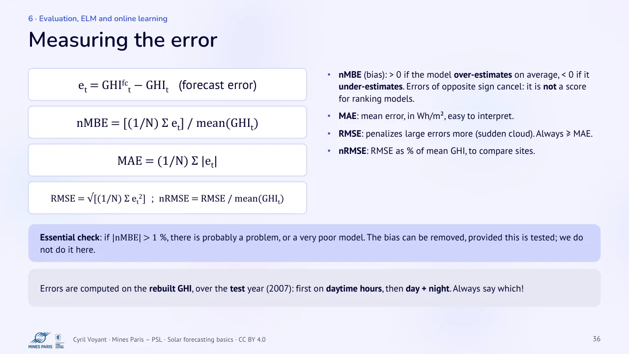
et = GHIfct − GHIt (forecast error)
nMBE = [(1/N) Σ et] / mean(GHIt)
MAE = (1/N) Σ |et|
RMSE = √[(1/N) Σ et2] ; nRMSE = RMSE / mean(GHIt)
Essential check: if |nMBE| > 1 %, there is probably a problem, or a very poor model. The bias can be removed, provided this is tested; we do not do it here.
Errors are computed on the rebuilt GHI, over the test year (2007): first on daytime hours, then day + night. Always say which!
nMBE (bias): > 0 if the model over-estimates on average, < 0 if it under-estimates. Errors of opposite sign cancel: it is not a score for ranking models.
MAE: mean error, in Wh/m², easy to interpret.
RMSE: penalizes large errors more (sudden cloud). Always ≥ MAE.
nRMSE: RMSE as % of mean GHI, to compare sites.
37 Comparing with persistence: SS and NICEΣ
Text of the slide
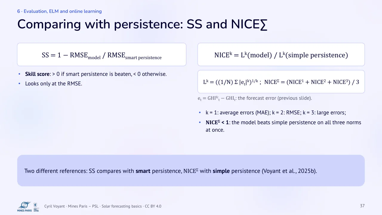
SS = 1 − RMSEmodel / RMSEsmart persistence
Skill score: > 0 if smart persistence is beaten, < 0 otherwise.
Looks only at the RMSE.
Two different references: SS compares with smart persistence, NICEΣ with simple persistence (Voyant et al., 2025b).
NICEk = Lk(model) / Lk(simple persistence)
Lk = ((1/N) Σ |et|k)1/k ; NICEΣ = (NICE1 + NICE2 + NICE3) / 3
et = GHIfct − GHIt: the forecast error (previous slide).
k = 1: average errors (MAE); k = 2: RMSE; k = 3: large errors;
NICEΣ < 1: the model beats simple persistence on all three norms at once.
38 Results at Ajaccio: 1-hour forecast
Text of the slide
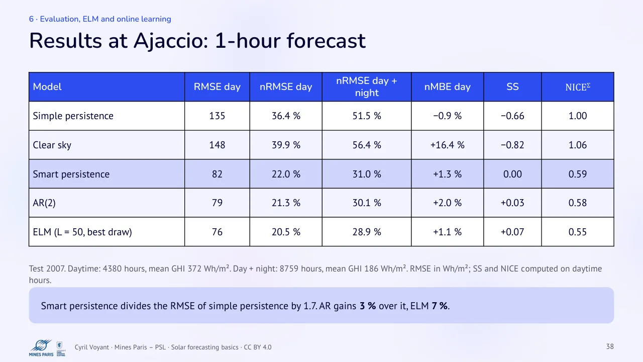
| Model | RMSE day | nRMSE day | nRMSE day + night | nMBE day | SS | NICEΣ |
|---|---|---|---|---|---|---|
| Simple persistence | 135 | 36.4 % | 51.5 % | −0.9 % | −0.66 | 1.00 |
| Clear sky | 148 | 39.9 % | 56.4 % | +16.4 % | −0.82 | 1.06 |
| Smart persistence | 82 | 22.0 % | 31.0 % | +1.3 % | 0.00 | 0.59 |
| AR(2) | 79 | 21.3 % | 30.1 % | +2.0 % | +0.03 | 0.58 |
| ELM (L = 50, best draw) | 76 | 20.5 % | 28.9 % | +1.1 % | +0.07 | 0.55 |
Test 2007. Daytime: 4380 hours, mean GHI 372 Wh/m². Day + night: 8759 hours, mean GHI 186 Wh/m². RMSE in Wh/m²; SS and NICE computed on daytime hours.
Smart persistence divides the RMSE of simple persistence by 1.7. AR gains 3 % over it, ELM 7 %.
39 Daytime only, or day + night?
Text of the slide
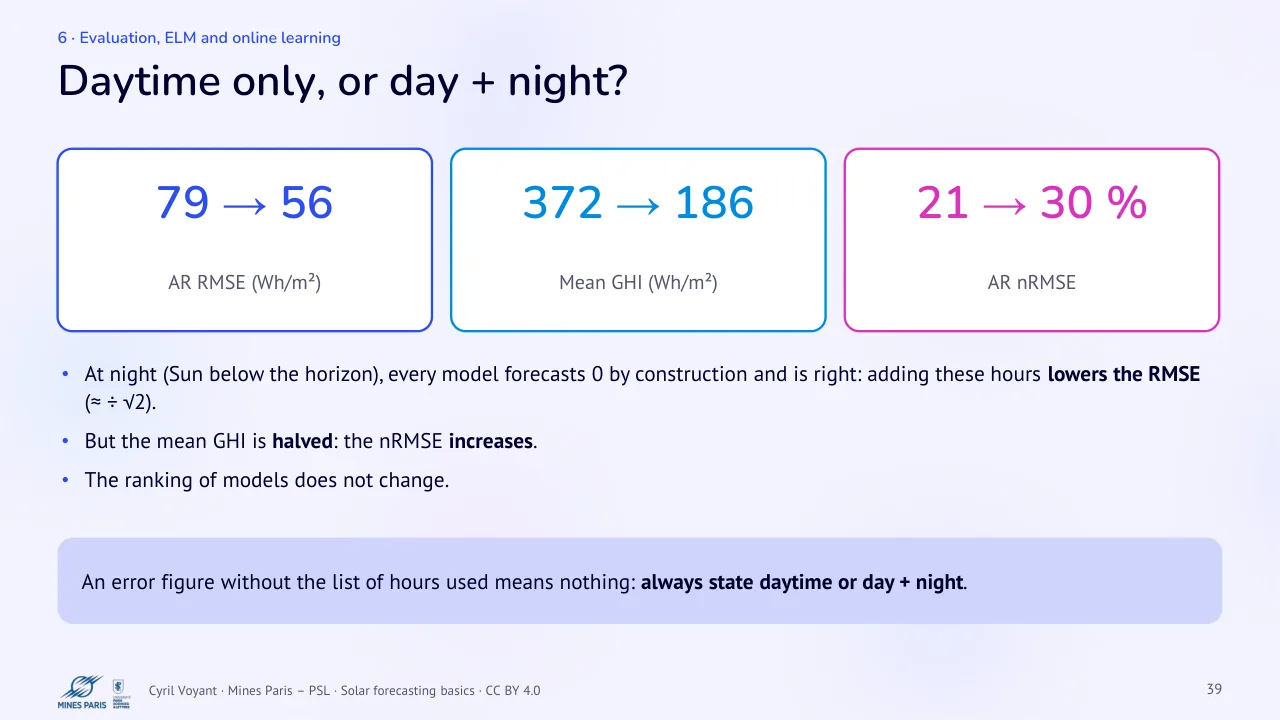
79 → 56 · AR RMSE (Wh/m²)
At night (Sun below the horizon), every model forecasts 0 by construction and is right: adding these hours lowers the RMSE (≈ ÷ √2).
But the mean GHI is halved: the nRMSE increases.
The ranking of models does not change.
An error figure without the list of hours used means nothing: always state daytime or day + night.
372 → 186
21 → 30 %
Mean GHI (Wh/m²) · AR nRMSE
40 The bias (nMBE): effect of the two rules
Text of the slide
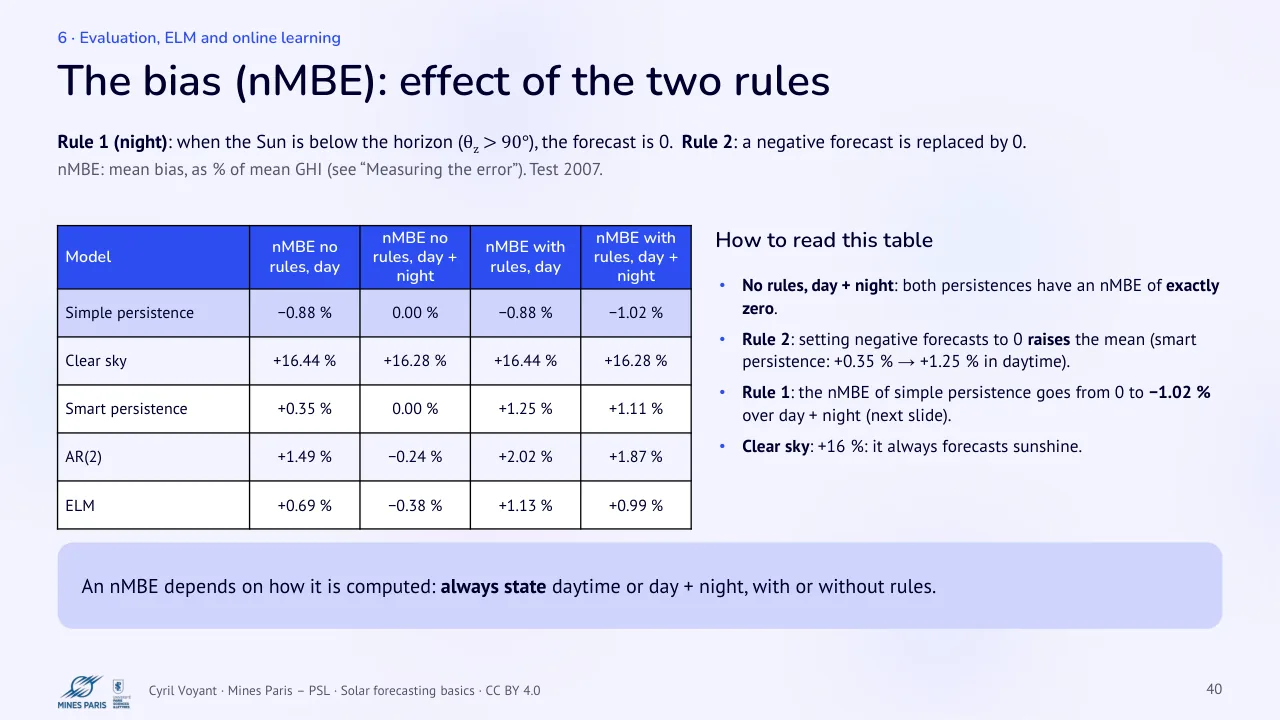
Rule 1 (night): when the Sun is below the horizon (θz > 90°), the forecast is 0. Rule 2: a negative forecast is replaced by 0.
nMBE: mean bias, as % of mean GHI (see “Measuring the error”). Test 2007.
| Model | nMBE no rules, day | nMBE no rules, day + night | nMBE with rules, day | nMBE with rules, day + night |
|---|---|---|---|---|
| Simple persistence | −0.88 % | 0.00 % | −0.88 % | −1.02 % |
| Clear sky | +16.44 % | +16.28 % | +16.44 % | +16.28 % |
| Smart persistence | +0.35 % | 0.00 % | +1.25 % | +1.11 % |
| AR(2) | +1.49 % | −0.24 % | +2.02 % | +1.87 % |
| ELM | +0.69 % | −0.38 % | +1.13 % | +0.99 % |
An nMBE depends on how it is computed: always state daytime or day + night, with or without rules.
How to read this table
No rules, day + night: both persistences have an nMBE of exactly zero.
Rule 2: setting negative forecasts to 0 raises the mean (smart persistence: +0.35 % → +1.25 % in daytime).
Rule 1: the nMBE of simple persistence goes from 0 to −1.02 % over day + night (next slide).
Clear sky: +16 %: it always forecasts sunshine.
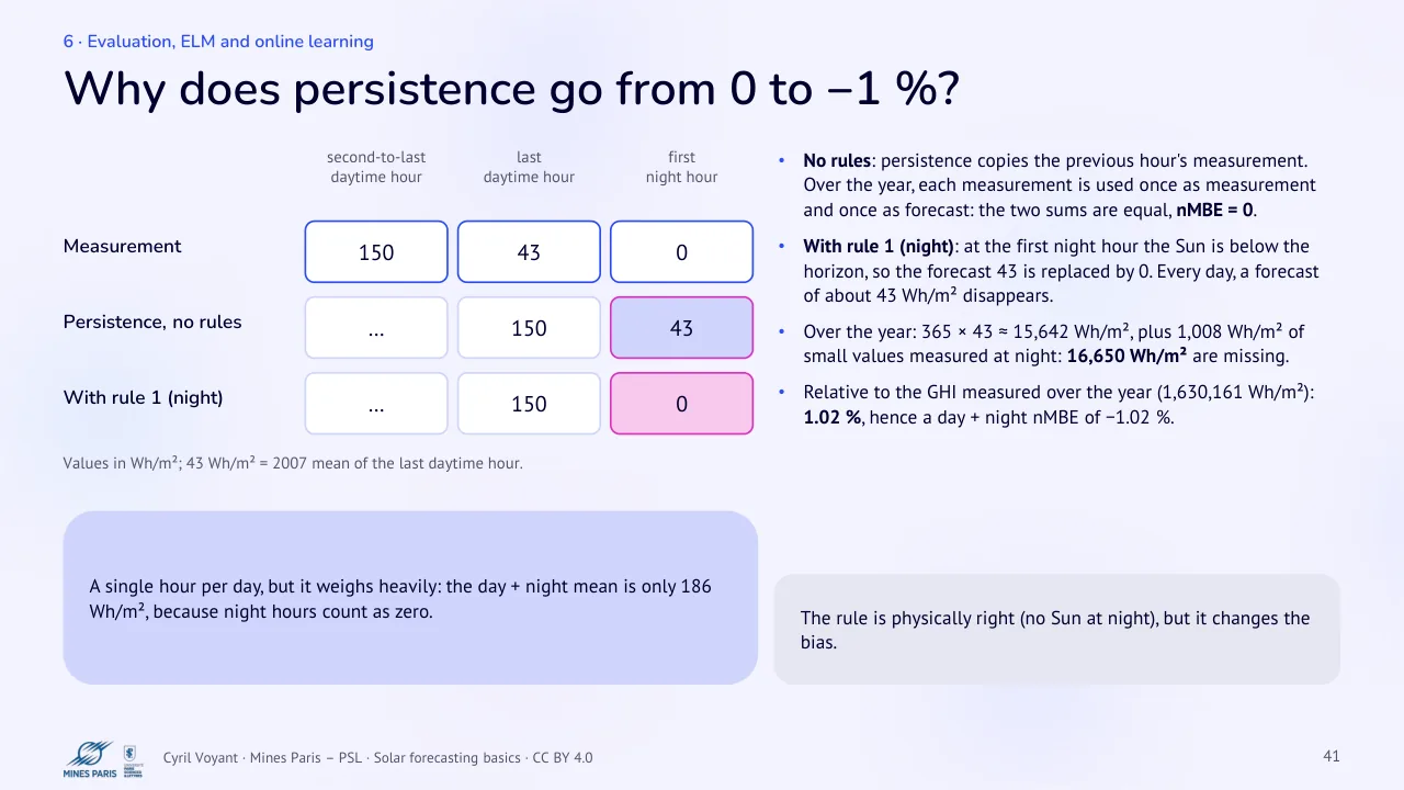
41 Why does persistence go from 0 to −1 %?
Text of the slide
second-to-last · daytime hour · last · daytime hour · 150 · 43 · Measurement · … · 150 · Persistence, no rules · … · 150
With rule 1 (night)
Values in Wh/m²; 43 Wh/m² = 2007 mean of the last daytime hour.
A single hour per day, but it weighs heavily: the day + night mean is only 186 Wh/m², because night hours count as zero.
first · night hour
No rules: persistence copies the previous hour's measurement. Over the year, each measurement is used once as measurement and once as forecast: the two sums are equal, nMBE = 0.
With rule 1 (night): at the first night hour the Sun is below the horizon, so the forecast 43 is replaced by 0. Every day, a forecast of about 43 Wh/m² disappears.
Over the year: 365 × 43 ≈ 15,642 Wh/m², plus 1,008 Wh/m² of small values measured at night: 16,650 Wh/m² are missing.
Relative to the GHI measured over the year (1,630,161 Wh/m²): 1.02 %, hence a day + night nMBE of −1.02 %.
0 · 43 · 0
The rule is physically right (no Sun at night), but it changes the bias.
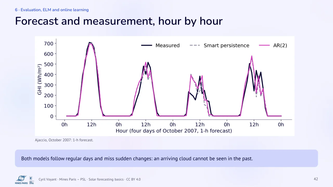
42 Forecast and measurement, hour by hour
Text of the slide
Ajaccio, October 2007: 1-h forecast.
Both models follow regular days and miss sudden changes: an arriving cloud cannot be seen in the past.
43 Limits of the AR model
Text of the slide
AR(p) assumes a linear relation between the CSI and its lags. Often enough at short horizons, but not always.
Difficult situations
fast clear / overcast transitions (cloud fronts);
cloud-edge effects (GHI > GHIcs);
very variable sky (cumulus);
nonlinear links between lags.
Under-fitting
A linear model cannot capture a curved relation, even with many lags.
Saturation
Beyond some p, adding lags no longer improves anything (slide “Choosing p”).
Idea: transform the inputs nonlinearly, then keep least squares. That is the ELM.
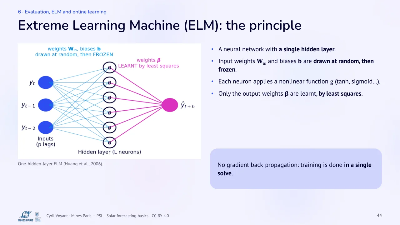
44 Extreme Learning Machine (ELM): the principle
Text of the slide
One-hidden-layer ELM (Huang et al., 2006).
A neural network with a single hidden layer.
Input weights Win and biases b are drawn at random, then frozen.
Each neuron applies a nonlinear function g (tanh, sigmoid…).
Only the output weights β are learnt, by least squares.
No gradient back-propagation: training is done in a single solve.
45 ELM: the formulation
Text of the slide
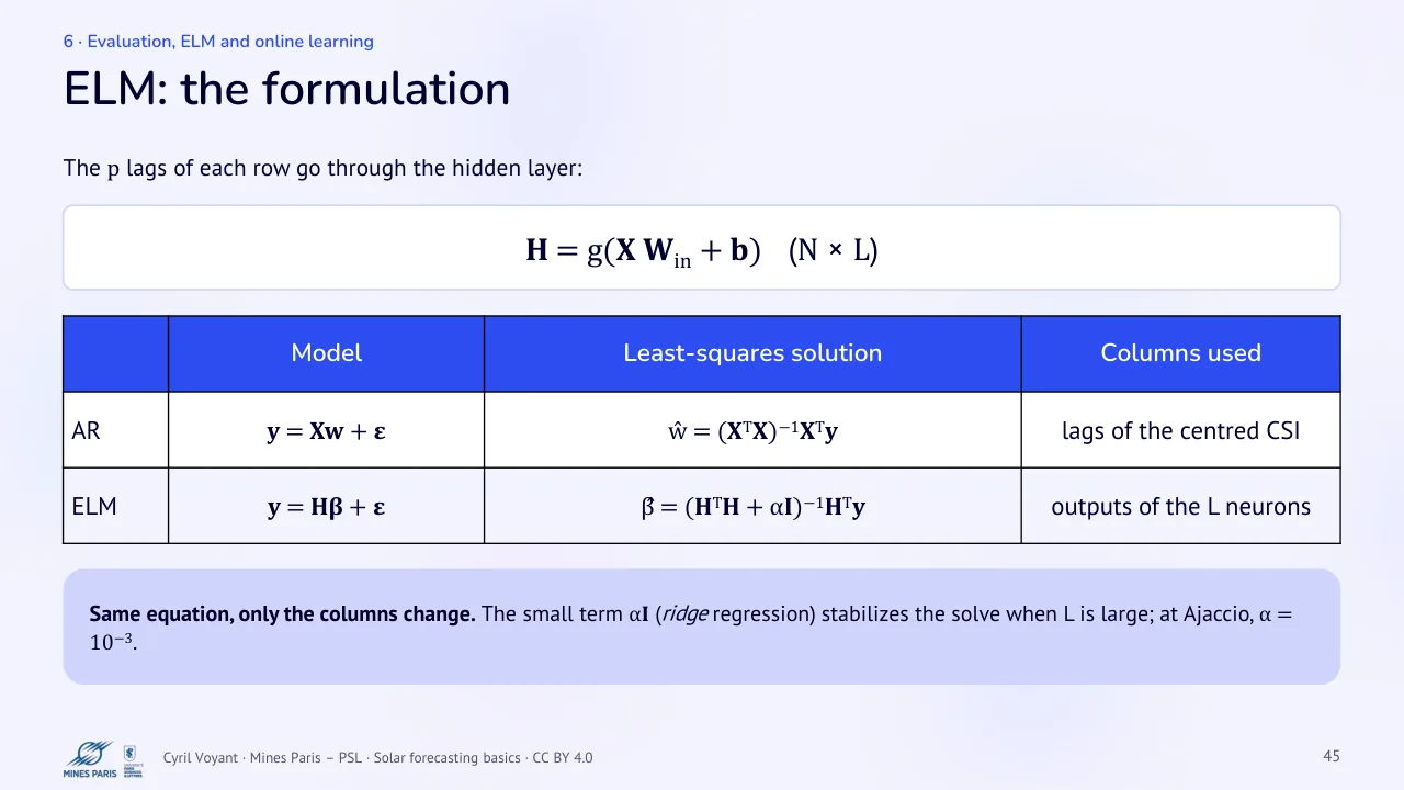
The p lags of each row go through the hidden layer:
H = g(X Win + b) (N × L)
| Model | Least-squares solution | Columns used | |
|---|---|---|---|
| AR | y = Xw + ε | ŵ = (XTX)−1XTy | lags of the centred CSI |
| ELM | y = Hβ + ε | β̂ = (HTH + αI)−1HTy | outputs of the L neurons |
Same equation, only the columns change. The small term αI (ridge regression) stabilizes the solve when L is large; at Ajaccio, α = 10−3.
46 ELM: choosing the number of neurons L
Text of the slide
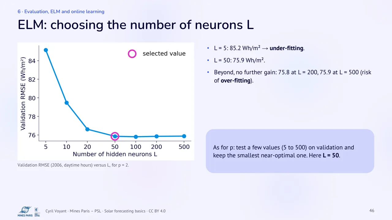
Validation RMSE (2006, daytime hours) versus L, for p = 2.
L = 5: 85.2 Wh/m² → under-fitting.
L = 50: 75.9 Wh/m².
Beyond, no further gain: 75.8 at L = 200, 75.9 at L = 500 (risk of over-fitting).
As for p: test a few values (5 to 500) on validation and keep the smallest near-optimal one. Here L = 50.
47 ELM: a result that depends on the draw
Text of the slide
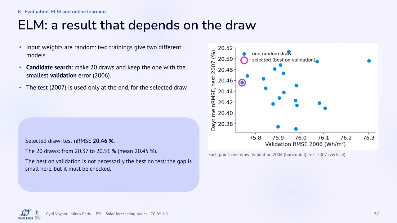
Input weights are random: two trainings give two different models.
Candidate search: make 20 draws and keep the one with the smallest validation error (2006).
The test (2007) is used only at the end, for the selected draw.
Selected draw: test nRMSE 20.46 %.
The 20 draws: from 20.37 to 20.51 % (mean 20.45 %).
The best on validation is not necessarily the best on test: the gap is small here, but it must be checked.
Each point: one draw. Validation 2006 (horizontal), test 2007 (vertical).
48 Giving the model the time: sin / cos encoding
Text of the slide
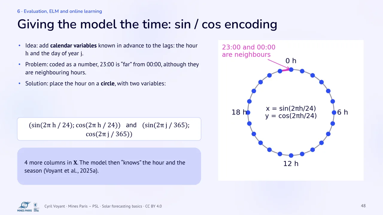
Idea: add calendar variables known in advance to the lags: the hour h and the day of year j.
Problem: coded as a number, 23:00 is “far” from 00:00, although they are neighbouring hours.
Solution: place the hour on a circle, with two variables:
(sin(2π h / 24); cos(2π h / 24)) and (sin(2π j / 365); cos(2π j / 365))
4 more columns in X. The model then “knows” the hour and the season (Voyant et al., 2025a).
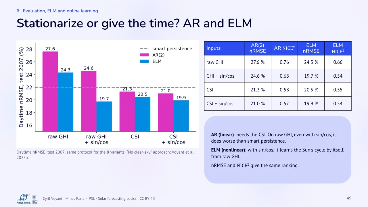
49 Stationarize or give the time? AR and ELM
Text of the slide
Daytime nRMSE, test 2007, same protocol for the 8 variants. “No clear-sky” approach: Voyant et al., 2025a.
| Inputs | AR(2) nRMSE | AR NICEΣ | ELM nRMSE | ELM NICEΣ |
|---|---|---|---|---|
| raw GHI | 27.6 % | 0.76 | 24.3 % | 0.66 |
| GHI + sin/cos | 24.6 % | 0.68 | 19.7 % | 0.54 |
| CSI | 21.3 % | 0.58 | 20.5 % | 0.55 |
| CSI + sin/cos | 21.0 % | 0.57 | 19.9 % | 0.54 |
AR (linear): needs the CSI. On raw GHI, even with sin/cos, it does worse than smart persistence.
ELM (nonlinear): with sin/cos, it learns the Sun's cycle by itself, from raw GHI.
nRMSE and NICEΣ give the same ranking.
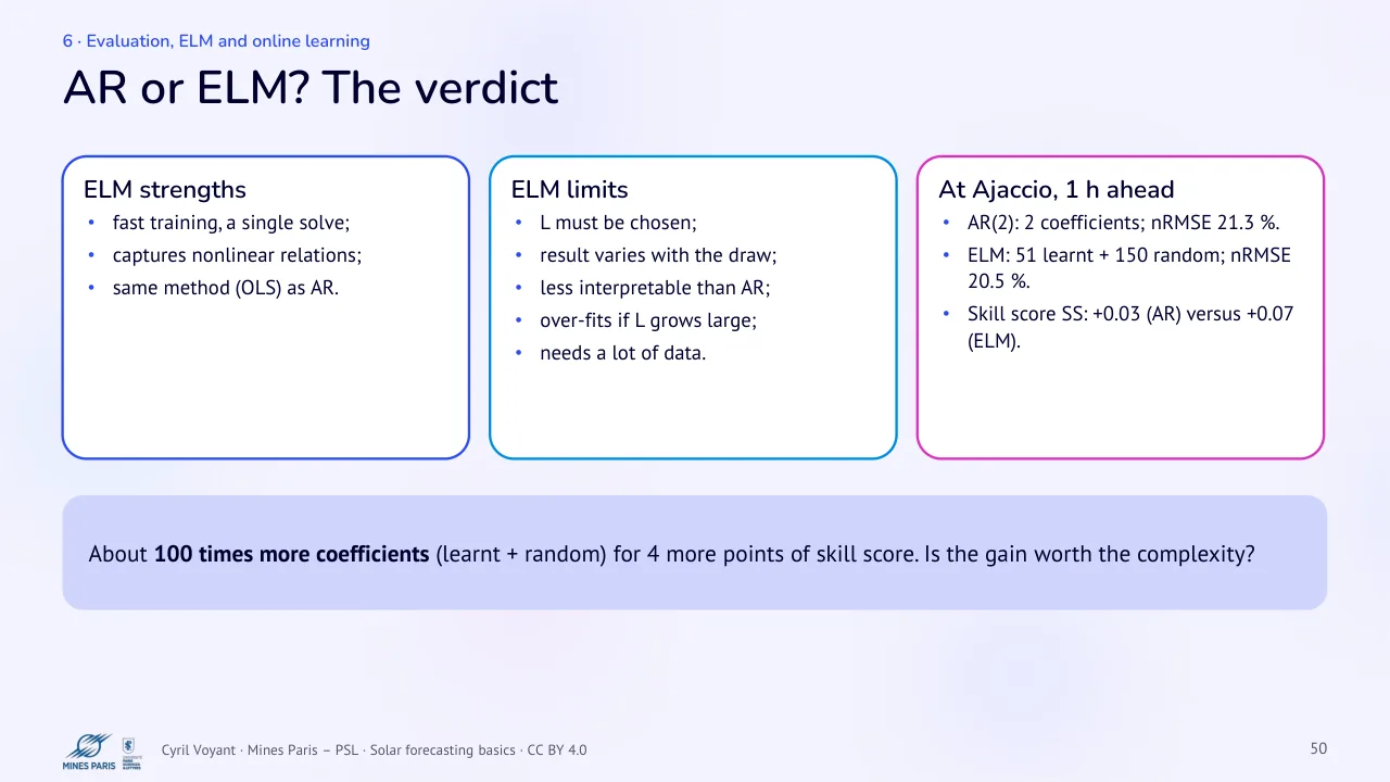
50 AR or ELM? The verdict
Text of the slide
ELM strengths
fast training, a single solve;
captures nonlinear relations;
same method (OLS) as AR.
About 100 times more coefficients (learnt + random) for 4 more points of skill score. Is the gain worth the complexity?
ELM limits
L must be chosen;
result varies with the draw;
less interpretable than AR;
over-fits if L grows large;
needs a lot of data.
At Ajaccio, 1 h ahead
AR(2): 2 coefficients; nRMSE 21.3 %.
ELM: 51 learnt + 150 random; nRMSE 20.5 %.
Skill score SS: +0.03 (AR) versus +0.07 (ELM).
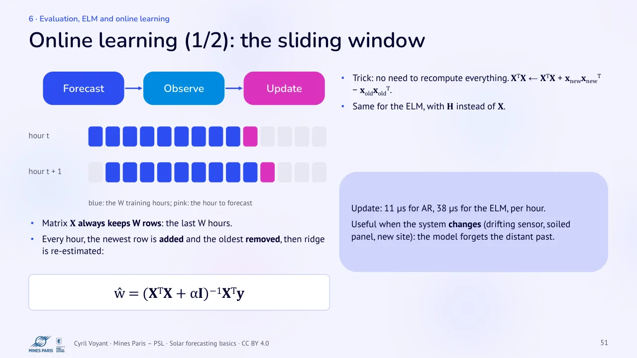
51 Online learning (1/2): the sliding window
Text of the slide
Forecast · Observe · hour t
hour t + 1
blue: the W training hours; pink: the hour to forecast
Matrix X always keeps W rows: the last W hours.
Every hour, the newest row is added and the oldest removed, then ridge is re-estimated:
ŵ = (XTX + αI)−1XTy
Update
Trick: no need to recompute everything. XTX ← XTX + xnewxnewT − xoldxoldT.
Same for the ELM, with H instead of X.
Update: 11 µs for AR, 38 µs for the ELM, per hour.
Useful when the system changes (drifting sensor, soiled panel, new site): the model forgets the distant past.
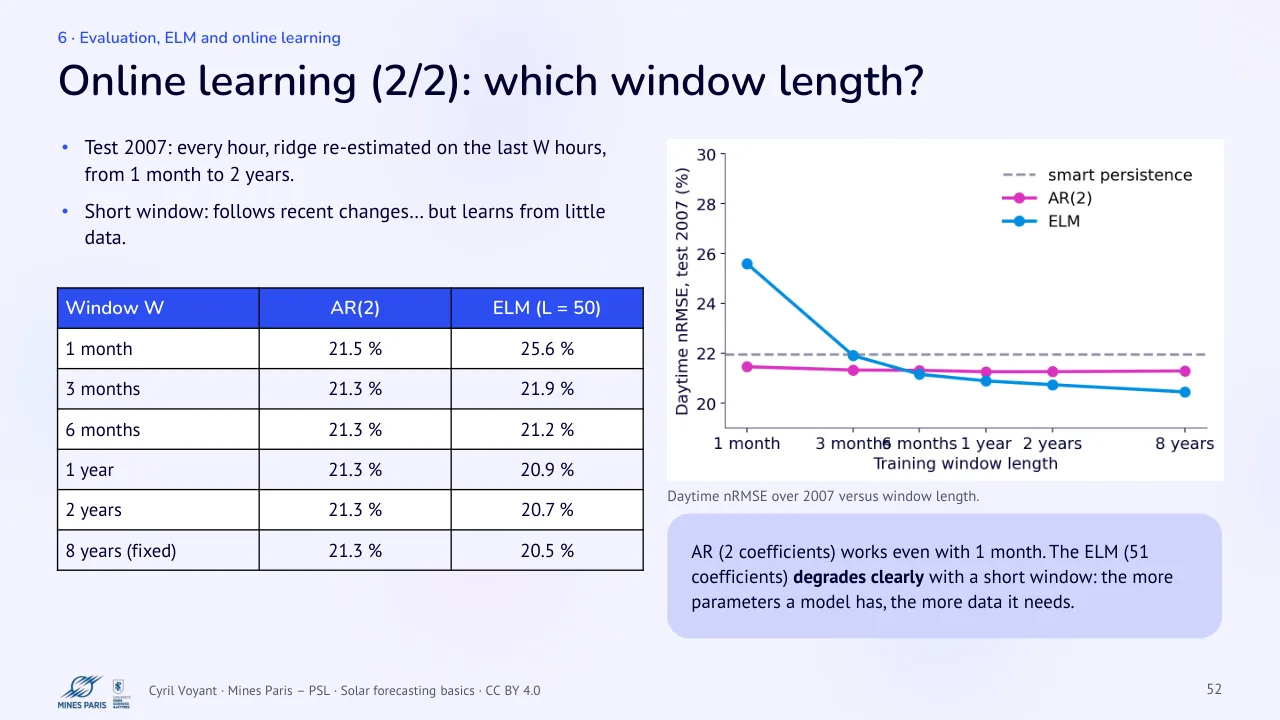
52 Online learning (2/2): which window length?
Text of the slide
Test 2007: every hour, ridge re-estimated on the last W hours, from 1 month to 2 years.
Short window: follows recent changes… but learns from little data.
| Window W | AR(2) | ELM (L = 50) |
|---|---|---|
| 1 month | 21.5 % | 25.6 % |
| 3 months | 21.3 % | 21.9 % |
| 6 months | 21.3 % | 21.2 % |
| 1 year | 21.3 % | 20.9 % |
| 2 years | 21.3 % | 20.7 % |
| 8 years (fixed) | 21.3 % | 20.5 % |
Daytime nRMSE over 2007 versus window length.
AR (2 coefficients) works even with 1 month. The ELM (51 coefficients) degrades clearly with a short window: the more parameters a model has, the more data it needs.
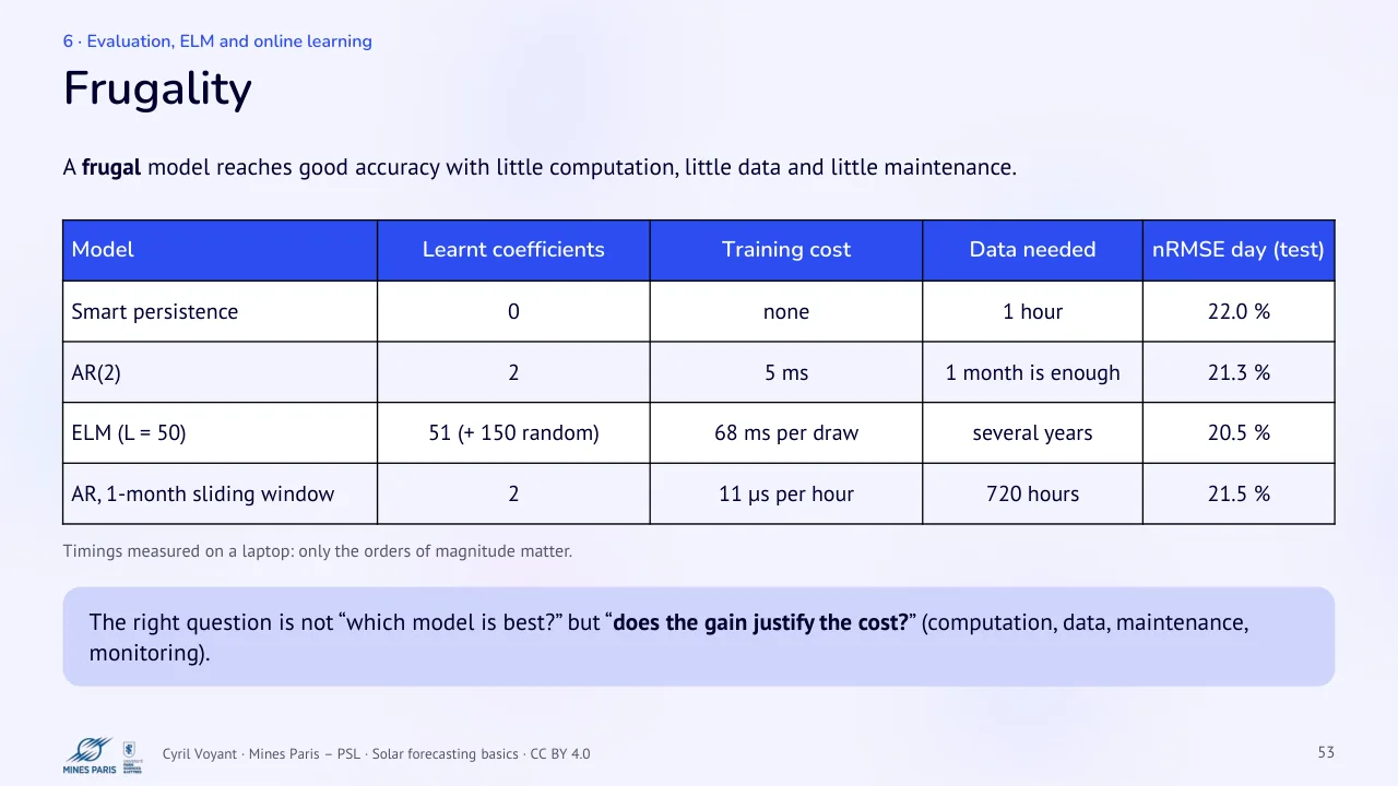
53 Frugality
Text of the slide
A frugal model reaches good accuracy with little computation, little data and little maintenance.
| Model | Learnt coefficients | Training cost | Data needed | nRMSE day (test) |
|---|---|---|---|---|
| Smart persistence | 0 | none | 1 hour | 22.0 % |
| AR(2) | 2 | 5 ms | 1 month is enough | 21.3 % |
| ELM (L = 50) | 51 (+ 150 random) | 68 ms per draw | several years | 20.5 % |
| AR, 1-month sliding window | 2 | 11 µs per hour | 720 hours | 21.5 % |
Timings measured on a laptop: only the orders of magnitude matter.
The right question is not “which model is best?” but “does the gain justify the cost?” (computation, data, maintenance, monitoring).
Project, glossary and references
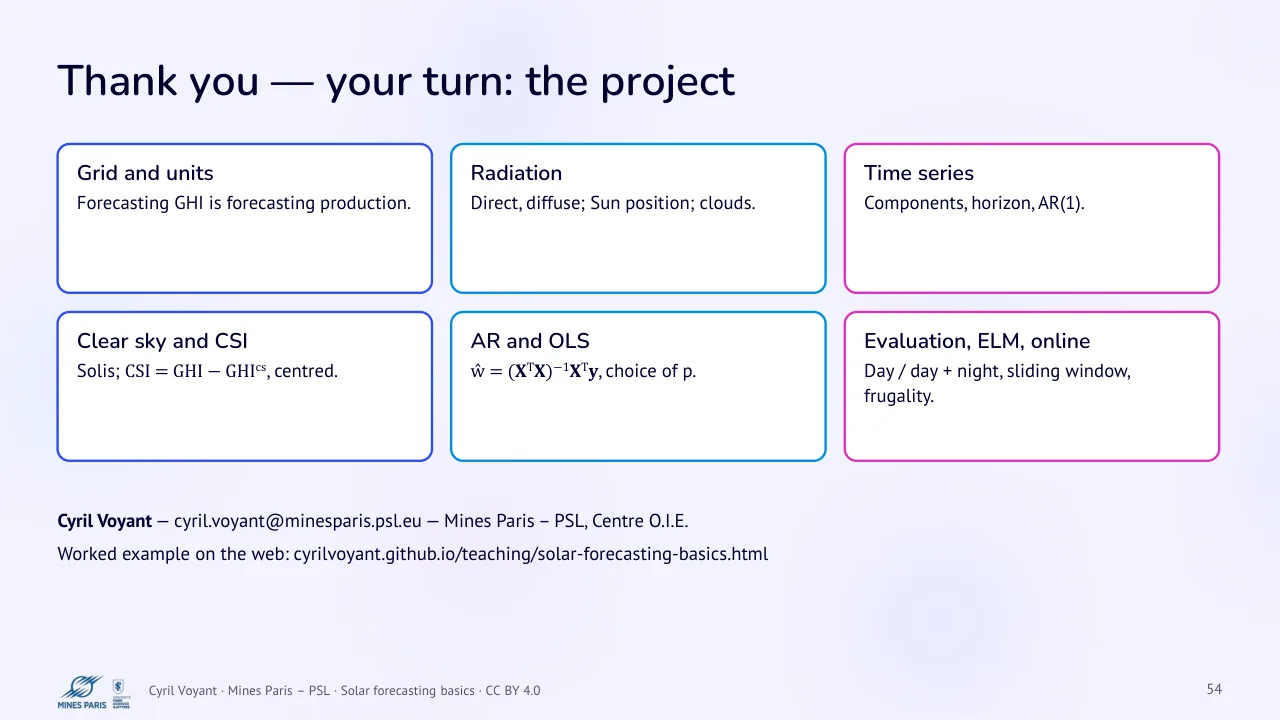
54 Thank you, your turn: the project
Text of the slide
Grid and units
Forecasting GHI is forecasting production.
Clear sky and CSI
Solis; CSI = GHI − GHIcs, centred.
Cyril Voyant (cyril.voyant@minesparis.psl.eu) Mines Paris – PSL, Centre O.I.E.
Worked example on the web: cyrilvoyant.github.io/teaching/solar-forecasting-basics.html
Radiation
Direct, diffuse; Sun position; clouds.
AR and OLS
ŵ = (XTX)−1XTy, choice of p.
Time series
Components, horizon, AR(1).
Evaluation, ELM, online
Day / day + night, sliding window, frugality.
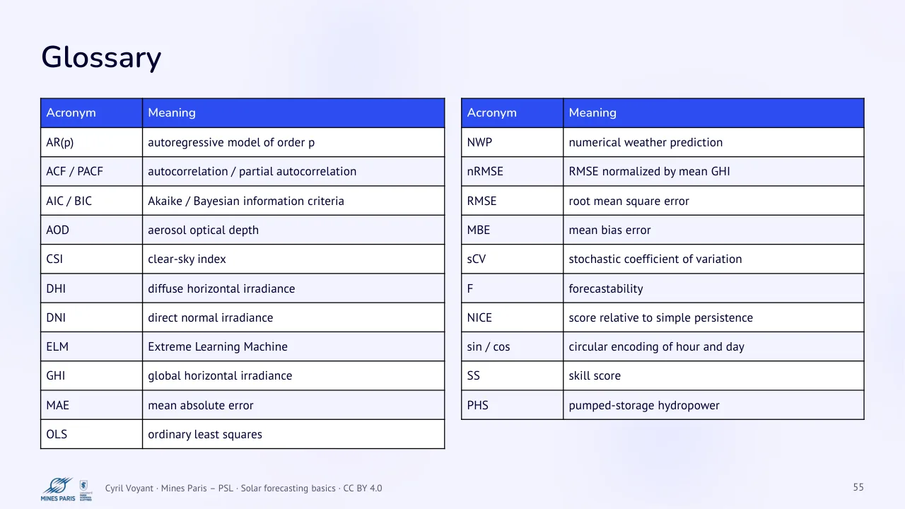
55 Glossary
Text of the slide
| Acronym | Meaning |
|---|---|
| AR(p) | autoregressive model of order p |
| ACF / PACF | autocorrelation / partial autocorrelation |
| AIC / BIC | Akaike / Bayesian information criteria |
| AOD | aerosol optical depth |
| CSI | clear-sky index |
| DHI | diffuse horizontal irradiance |
| DNI | direct normal irradiance |
| ELM | Extreme Learning Machine |
| GHI | global horizontal irradiance |
| MAE | mean absolute error |
| OLS | ordinary least squares |
| Acronym | Meaning |
|---|---|
| NWP | numerical weather prediction |
| nRMSE | RMSE normalized by mean GHI |
| RMSE | root mean square error |
| MBE | mean bias error |
| sCV | stochastic coefficient of variation |
| F | forecastability |
| NICE | score relative to simple persistence |
| sin / cos | circular encoding of hour and day |
| SS | skill score |
| PHS | pumped-storage hydropower |
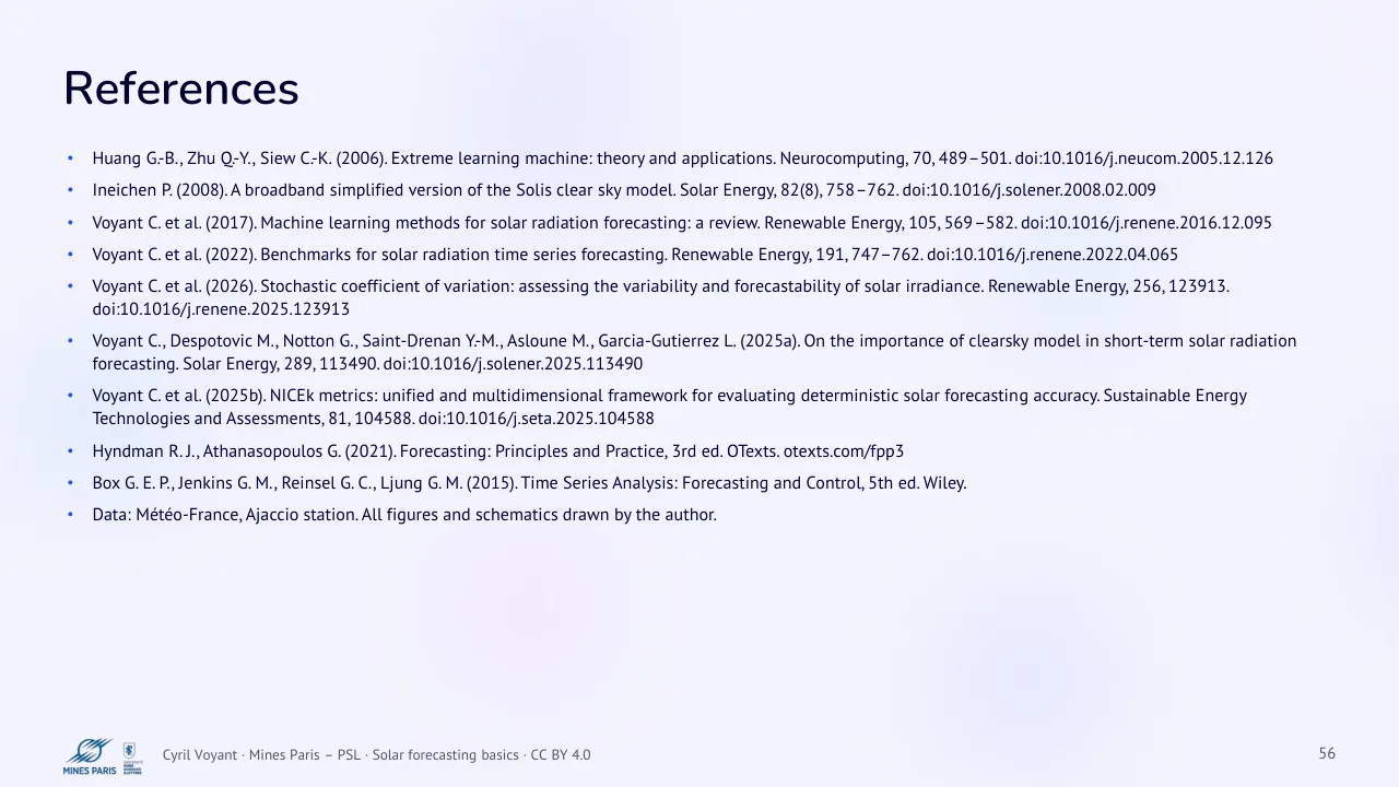
56 References
Text of the slide
Huang G.-B., Zhu Q.-Y., Siew C.-K. (2006). Extreme learning machine: theory and applications. Neurocomputing, 70, 489–501. doi:10.1016/j.neucom.2005.12.126
Ineichen P. (2008). A broadband simplified version of the Solis clear sky model. Solar Energy, 82(8), 758–762. doi:10.1016/j.solener.2008.02.009
Voyant C. et al. (2017). Machine learning methods for solar radiation forecasting: a review. Renewable Energy, 105, 569–582. doi:10.1016/j.renene.2016.12.095
Voyant C. et al. (2022). Benchmarks for solar radiation time series forecasting. Renewable Energy, 191, 747–762. doi:10.1016/j.renene.2022.04.065
Voyant C. et al. (2026). Stochastic coefficient of variation: assessing the variability and forecastability of solar irradiance. Renewable Energy, 256, 123913. doi:10.1016/j.renene.2025.123913
Voyant C., Despotovic M., Notton G., Saint-Drenan Y.-M., Asloune M., Garcia-Gutierrez L. (2025a). On the importance of clearsky model in short-term solar radiation forecasting. Solar Energy, 289, 113490. doi:10.1016/j.solener.2025.113490
Voyant C. et al. (2025b). NICEk metrics: unified and multidimensional framework for evaluating deterministic solar forecasting accuracy. Sustainable Energy Technologies and Assessments, 81, 104588. doi:10.1016/j.seta.2025.104588
Hyndman R. J., Athanasopoulos G. (2021). Forecasting: Principles and Practice, 3rd ed. OTexts. otexts.com/fpp3
Box G. E. P., Jenkins G. M., Reinsel G. C., Ljung G. M. (2015). Time Series Analysis: Forecasting and Control, 5th ed. Wiley.
Data: Météo-France, Ajaccio station. All figures and schematics drawn by the author.
Appendices
57 Appendix A, Wide-sense stationarity
Text of the slide
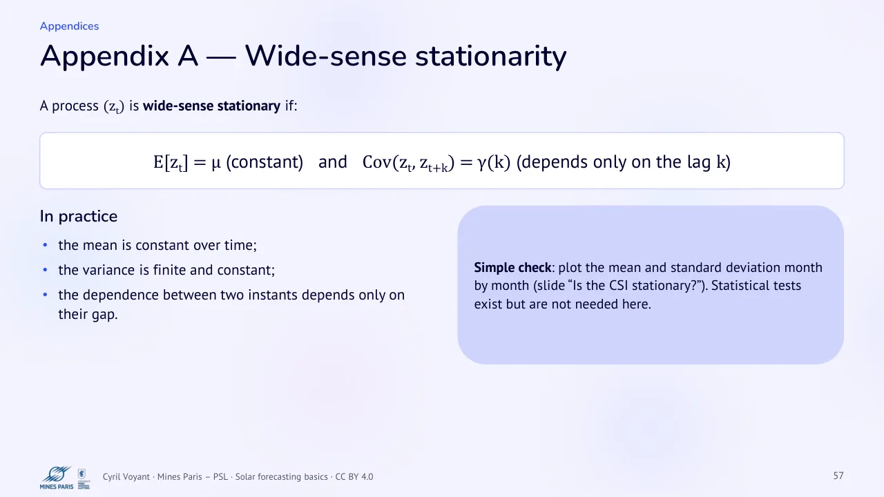
A process (zt) is wide-sense stationary if:
E[zt] = μ (constant) and Cov(zt, zt+k) = γ(k) (depends only on the lag k)
In practice
the mean is constant over time;
the variance is finite and constant;
the dependence between two instants depends only on their gap.
Simple check: plot the mean and standard deviation month by month (slide “Is the CSI stationary?”). Statistical tests exist but are not needed here.
58 Appendix B, The best possible forecast
Text of the slide
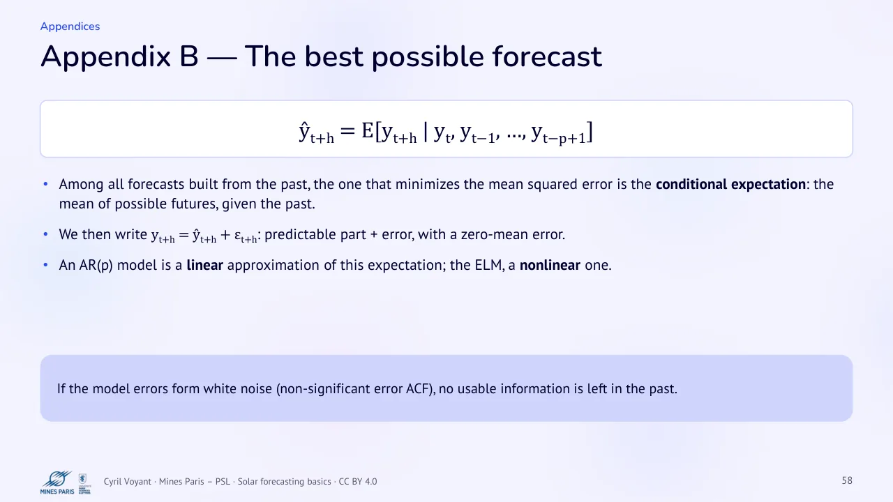
ŷt+h = E[yt+h | yt, yt−1, …, yt−p+1]
Among all forecasts built from the past, the one that minimizes the mean squared error is the conditional expectation: the mean of possible futures, given the past.
We then write yt+h = ŷt+h + εt+h: predictable part + error, with a zero-mean error.
An AR(p) model is a linear approximation of this expectation; the ELM, a nonlinear one.
If the model errors form white noise (non-significant error ACF), no usable information is left in the past.
59 Appendix C, Choosing p with AIC or BIC
Text of the slide
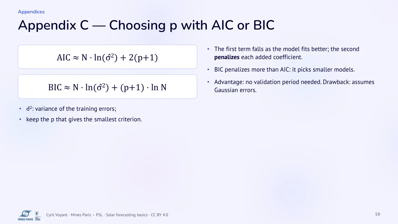
AIC ≈ N · ln(σ̂2) + 2(p+1)
BIC ≈ N · ln(σ̂2) + (p+1) · ln N
σ̂2: variance of the training errors;
keep the p that gives the smallest criterion.
The first term falls as the model fits better; the second penalizes each added coefficient.
BIC penalizes more than AIC: it picks smaller models.
Advantage: no validation period needed. Drawback: assumes Gaussian errors.
Go further
- Solar forecasting basics: the whole course as a worked example, with equations, real numbers and code.
- Course summary and questions answered on the methods site.
- Worked examples: stochastic persistence · BLEND · persistence, AR and ELM compared.
- Research behind the course: sCV and F · NICE metrics · BLEND · all stories.